Weighted Tidy Log Odds Ratio.

tidylo: Weighted Tidy Log Odds Ratio ⚖️

Authors:Julia Silge, Alex Hayes, Tyler Schnoebelen
License:MIT

How can we measure how the usage or frequency of some feature, such as words, differs across some group or set, such as documents? One option is to use the log odds ratio, but the log odds ratio alone does not account for sampling variability; we haven’t counted every feature the same number of times so how do we know which differences are meaningful?

Enter the weighted log odds, which tidylo provides an implementation for, using tidy data principles. In particular, here we use the method outlined in Monroe, Colaresi, and Quinn (2008) to weight the log odds ratio by a prior. By default, the prior is estimated from the data itself, an empirical Bayes approach, but an uninformative prior is also available.

Installation

You can install the released version of tidylo from CRAN with:

install.packages("tidylo")

Or you can install the development version from GitHub with devtools:

# install.packages("devtools")
devtools::install_github("juliasilge/tidylo")

Example

Using weighted log odds is a great approach for text analysis when we want to measure how word usage differs across a set of documents. Let’s explore the six published, completed novels of Jane Austen and use the tidytext package to count up the bigrams (sequences of two adjacent words) in each novel. This weighted log odds approach would work equally well for single words.

library(dplyr)
#> 
#> Attaching package: 'dplyr'
#> The following objects are masked from 'package:stats':
#> 
#>     filter, lag
#> The following objects are masked from 'package:base':
#> 
#>     intersect, setdiff, setequal, union
library(janeaustenr)
library(tidytext)

tidy_bigrams <- austen_books() %>%
    unnest_tokens(bigram, text, token = "ngrams", n = 2) %>%
    filter(!is.na(bigram))

bigram_counts <- tidy_bigrams %>%
    count(book, bigram, sort = TRUE)

bigram_counts
#> # A tibble: 300,903 × 3
#>    book                bigram     n
#>    <fct>               <chr>  <int>
#>  1 Mansfield Park      of the   712
#>  2 Mansfield Park      to be    612
#>  3 Emma                to be    586
#>  4 Mansfield Park      in the   533
#>  5 Emma                of the   529
#>  6 Pride & Prejudice   of the   439
#>  7 Emma                it was   430
#>  8 Pride & Prejudice   to be    422
#>  9 Sense & Sensibility to be    418
#> 10 Emma                in the   416
#> # … with 300,893 more rows

Now let’s use the bind_log_odds() function from the tidylo package to find the weighted log odds for each bigram. The weighted log odds computed by this function are also z-scores for the log odds; this quantity is useful for comparing frequencies across categories or sets but its relationship to an odds ratio is not straightforward after the weighting.

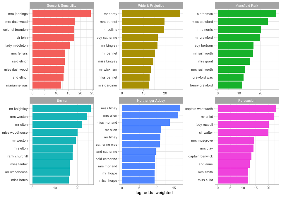
What are the bigrams with the highest weighted log odds for these books?

library(tidylo)

bigram_log_odds <- bigram_counts %>%
    bind_log_odds(book, bigram, n) 

bigram_log_odds %>%
    arrange(-log_odds_weighted)
#> # A tibble: 300,903 × 4
#>    book                bigram                n log_odds_weighted
#>    <fct>               <chr>             <int>             <dbl>
#>  1 Mansfield Park      sir thomas          266              27.2
#>  2 Pride & Prejudice   mr darcy            230              27.0
#>  3 Emma                mr knightley        239              25.9
#>  4 Sense & Sensibility mrs jennings        185              24.3
#>  5 Emma                mrs weston          208              24.2
#>  6 Mansfield Park      miss crawford       196              23.4
#>  7 Persuasion          captain wentworth   143              23.0
#>  8 Persuasion          mr elliot           133              22.2
#>  9 Emma                mr elton            174              22.1
#> 10 Mansfield Park      mrs norris          148              20.3
#> # … with 300,893 more rows

The bigrams more likely to come from each book, compared to the others, involve proper nouns. We can make a visualization as well.

library(ggplot2)

bigram_log_odds %>%
    group_by(book) %>%
    slice_max(log_odds_weighted, n = 10) %>%
    ungroup() %>%
    mutate(bigram = reorder(bigram, log_odds_weighted)) %>%
    ggplot(aes(log_odds_weighted, bigram, fill = book)) +
    geom_col(show.legend = FALSE) +
    facet_wrap(vars(book), scales = "free") +
    labs(y = NULL)

Community Guidelines

This project is released with a Contributor Code of Conduct. By contributing to this project, you agree to abide by its terms. Feedback, bug reports (and fixes!), and feature requests are welcome; file issues or seek support here.