r-ARCensReg

Fitting Univariate Censored Linear Regression Model with Autoregressive Errors.

The ARCensReg R package

The ARCensReg package fits a univariate censored linear regression model with autoregressive (AR) errors. The discrete-time representation of this model for the observed response at time t is given by

Y_t = x_t^⊤β + ξ_t,

ξ_t = ϕ₁ξ_t − 1 + ϕ₂ξ_t − 2 + ... + ϕ_pξ_t − p + η_t,  t = 1, ..., p, p + 1, ..., n,

where Y_t is the response variable, β is a vector of regression parameters of dimension l, x_t is a vector of non-stochastic regressor variables, and ξ_t is the AR error with η_t representing the innovations and ϕ denoting the vector of AR coefficients. For the innovations η_t, we consider the normal or the Student-t distribution. The maximum likelihood estimates are obtained through the Stochastic Approximation Expectation-Maximization (SAEM) algorithm (Delyon, Lavielle, and Moulines 1999), while the standard errors of the parameters are approximated by the Louis method (Louis 1982). This package also predicts future observations and supports missing values on the dependent variable. See, for instance, (Schumacher, Lachos, and Dey 2017) and (Valeriano et al. 2021).

For the normal model, influence diagnostic could be performed by a local influence approach (Cook 1986) with three possible perturbation schemes: response perturbation, scale matrix perturbation, or explanatory variable perturbation. For more details see (Schumacher et al. 2018).

The ARCensReg package provides the following functions:

• ARCensReg: fits a univariate censored linear regression model with autoregressive errors under the normal distribution.
• ARtCensReg: fits a univariate censored linear regression model with autoregressive errors considering Student-t innovations.
• InfDiag: performs influence diagnostic by a local influence approach with three possible perturbation schemes.
• rARCens: simulates a censored response variable with autoregressive errors of order p.
• residuals: computes conditional and quantile residuals.

predict, print, summary, and plot functions also work for objects given as an output of functions ARCensReg and ARtCensReg. Function plot also has methods for outputs of functions InfDiag and residuals.

Next, we will describe how to install the package and use all the previous methods in artificial examples.

Installation

The released version of ARCensReg from CRAN can be installed with:

install.packages("ARCensReg")

And the development version from GitHub with:

# install.packages("devtools")
devtools::install_github("fernandalschumacher/ARCensReg")

Examples

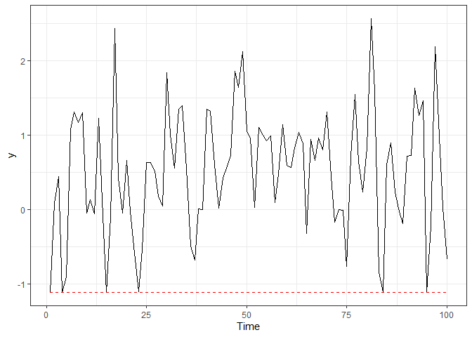
Example 1. We simulated a dataset of length n = 100 from the autoregressive model of order p = 2 with normal innovations and left censoring.

library(ARCensReg)
library(ggplot2)

set.seed(12341)
n = 100
x = cbind(1, runif(n))
dat = rARCens(n=n, beta=c(1,-1), phi=c(.48,-0.4), sig2=.5, x=x,
              cens='left', pcens=.05, innov="norm")

ggplot(dat$data, aes(x=1:n, y=y)) + geom_line() + labs(x="Time") + theme_bw() +
  geom_line(aes(x=1:n, y=ucl), color="red", linetype="dashed")

Supposing the AR order is unknown, we fit a censored linear regression model with Gaussian AR errors of order p = 1 and p = 2, and the information criteria are compared.

fit1 = ARCensReg(dat$data$cc, dat$data$lcl, dat$data$ucl, dat$data$y, x, 
                 p=1, pc=0.15, show_se=FALSE, quiet=TRUE)
fit1$critFin 
#>         Loglik     AIC     BIC AICcorr
#> Value -113.027 234.054 244.475 234.475

fit2 = ARCensReg(dat$data$cc, dat$data$lcl, dat$data$ucl, dat$data$y, x, 
                 p=2, pc=0.15, quiet=TRUE)
fit2$critFin
#>         Loglik     AIC     BIC AICcorr
#> Value -105.279 220.558 233.583 221.196

Based on the information criteria AIC and BIC, the model with AR errors of order p = 2 is the best fit for this data. The parameter estimates and standard errors can be visualized through functions summary and print.

summary(fit2)
#> ---------------------------------------------------
#>   Censored Linear Regression Model with AR Errors 
#> ---------------------------------------------------
#> Call:
#> ARCensReg(cc = dat$data$cc, lcl = dat$data$lcl, ucl = dat$data$ucl, 
#>     y = dat$data$y, x = x, p = 2, pc = 0.15, quiet = TRUE)
#> 
#> Estimated parameters:
#>       beta0   beta1 sigma2   phi1    phi2
#>      1.0830 -1.0965 0.4713 0.4690 -0.3883
#> s.e. 0.1465  0.2389 0.0689 0.0949  0.0941
#> 
#> Model selection criteria:
#>         Loglik     AIC     BIC AICcorr
#> Value -105.279 220.558 233.583 221.196
#> 
#> Details:
#> Type of censoring: left 
#> Number of missing values: 0 
#> Convergence reached?:  
#> Iterations: 168 / 400 
#> MC sample: 10 
#> Cut point: 0.15 
#> Processing time: 44.76831 secs

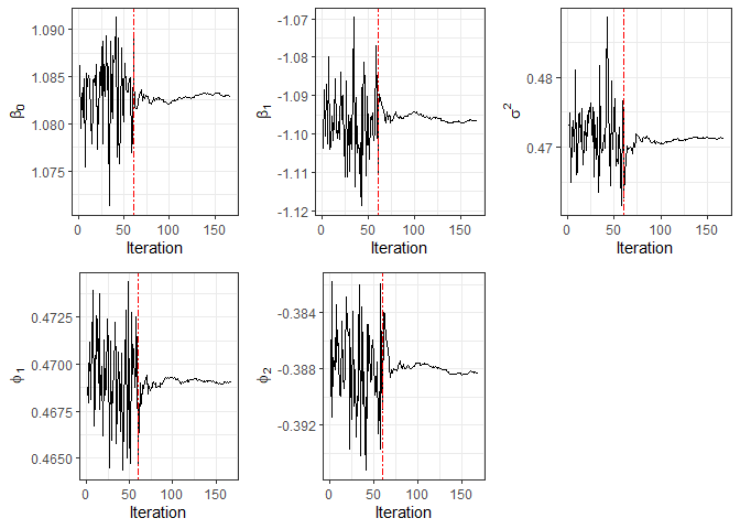
Moreover, for censored data, the convergence plot of the parameter estimates can be displayed through function plot.

plot(fit2)

Now, we perturb the observation 81 by making it equal to 6 and then fit a censored linear regression model with Gaussian AR errors of order p = 2.

y2 = dat$data$y
y2[81] = 6
fit3 = ARCensReg(dat$data$cc, dat$data$lcl, dat$data$ucl, y2, x, p=2,
                 show_se=FALSE, quiet=TRUE)
fit3$tab
#>   beta0   beta1 sigma2   phi1    phi2
#>  1.1702 -1.2065 0.7237 0.3812 -0.3355

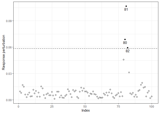
It is worth noting that the parameter estimates were affected because of the perturbation. Thence, we can perform influence diagnostic to identify influential points which may cause unwanted effects on estimation and goodness of fit. In the following analysis, we only consider the response perturbation scheme, where we deduced that observations 80 to 82 may be influential.

M0y = InfDiag(fit3, k=3.5, perturbation="y")
#> Perturbation scheme: y 
#> Benchmark: 0.059 
#> Detected points: 80 81 82
plot(M0y)

Example 2. A dataset of size n = 200 is simulated from the censored regression model with Student-t innovations and right censoring. To fit this data, we can use the function ARtCensReg, but it is worth mentioning that this function only works for response vectors with the first p values wholly observed.

set.seed(783796)
n = 200
x = cbind(1, runif(n))
dat2 = rARCens(n=n, beta=c(2,1), phi=c(.48,-.2), sig2=.5, x=x, cens='right',
               pcens=.05, innov='t', nu=3)
head(dat2$data)
#>           y cc      lcl ucl
#> 1 3.3242078  0 4.284143 Inf
#> 2 2.9409784  0 4.284143 Inf
#> 3 3.5386525  0 4.284143 Inf
#> 4 3.4107191  0 4.284143 Inf
#> 5 0.3564079  0 4.284143 Inf
#> 6 2.6332103  0 4.284143 Inf

For models with Student-t innovations, the degrees of freedom can be provided through argument nufix when it is known, or the algorithm will estimate it when it is not provided, i.e., nufix=NULL.

# Fitting the model with nu known
fit1 = ARtCensReg(dat2$data$cc, dat2$data$lcl, dat2$data$ucl, dat2$data$y, x,
                  p=2, M=20, nufix=3, quiet=TRUE)
fit1$tab
#>       beta0  beta1 sigma2   phi1    phi2
#>      1.9707 0.9594 0.4468 0.3778 -0.1562
#> s.e. 0.1230 0.1890 0.0640 0.0572  0.0590

# Fitting the model with nu unknown
fit2 = ARtCensReg(dat2$data$cc, dat2$data$lcl, dat2$data$ucl, dat2$data$y, x,
                  p=2, M=20, quiet=TRUE)
fit2$tab
#>       beta0  beta1 sigma2   phi1    phi2     nu
#>      1.9630 0.9720 0.4812 0.3798 -0.1563 3.4760
#> s.e. 0.1266 0.1953 0.0991 0.0592  0.0606 1.1295

Note that the parameter estimates obtained from both models are close, and the estimate of ν was close to the true value (ν = 3).

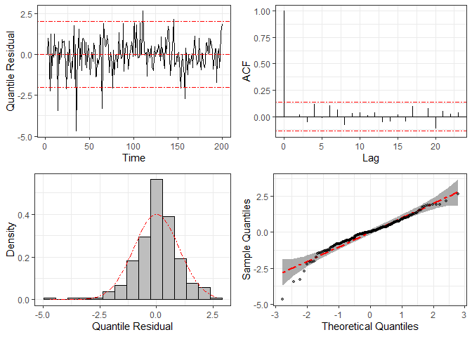
To check the statistical model’s specification, we can use graphical methods based on the quantile residuals, which are computed through function residuals and plotted by function plot.

res = residuals(fit2)
plot(res)

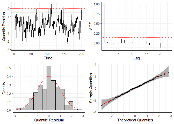
For comparison, we fit the same dataset considering the normal distribution (i.e., disregarding the heavy tails) and compute the corresponding quantile residuals. The resulting plots are given below, where we can see clear signs of non-normality, such as large residuals and some points outside the confidence band in the Q-Q plots.

fit3 = ARCensReg(dat2$data$cc, dat2$data$lcl, dat2$data$ucl, dat2$data$y, x,
                 p=2, M=20, show_se=FALSE, quiet=TRUE)
plot(residuals(fit3))

References

Cook, R. D. 1986. “Assessment of Local Influence.” Journal of the Royal Statistical Society: Series B (Methodological) 48 (2): 133–55.
Delyon, B., M. Lavielle, and E. Moulines. 1999. “Convergence of a Stochastic Approximation Version of the EM Algorithm.” Annals of Statistics, 94–128.
Louis, T. A. 1982. “Finding the Observed Information Matrix When Using the EM Algorithm.” Journal of the Royal Statistical Society: Series B (Methodological) 44 (2): 226–33.
Schumacher, F. L., V. H. Lachos, and D. K. Dey. 2017. “Censored Regression Models with Autoregressive Errors: A Likelihood-Based Perspective.” Canadian Journal of Statistics 45 (4): 375–92.
Schumacher, F. L., V. H. Lachos, F. E. Vilca-Labra, and L. M. Castro. 2018. “Influence Diagnostics for Censored Regression Models with Autoregressive Errors.” Australian & New Zealand Journal of Statistics 60 (2): 209–29.
Valeriano, K. L., F. L. Schumacher, C. E. Galarza, and L. A. Matos. 2021. “Censored Autoregressive Regression Models with Student-t Innovations.” arXiv Preprint arXiv:2110.00224.