Description
Babson Analytics and Quantitative Methods Tools.
Description
Instructor-developed tools for Analytics and Quantitative Methods (AQM) courses at Babson College. Included are compact descriptive statistics for data frames and lists, expanded reporting and graphics for linear regressions, and formatted reports for best subsets analyses.
README.md
BAQM
![]()
BAQM supplies functions developed by Babson College instructors for AQM 1000 and AQM 2000 courses using R in the curriculum. The primary functions provide:
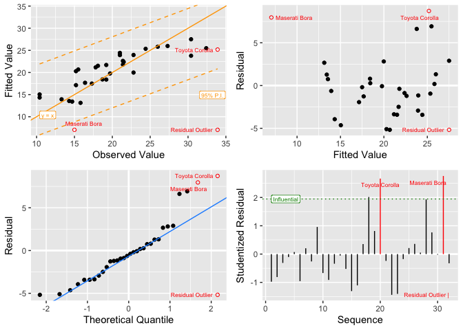
sumry.df()- summary descriptive statistics for data frames, allowing both numeric and factor variables, in both wide and long formats.sumry.lm()- expanded statistics and enhanced formatting to summarize linear model results.lm_plot.4way()- multiple diagnostic plots for linear models using ggplot, including a 4-in-1 summary graphic.sumry.regsubsets()- compact “best subsets” linear model reports for analytics from theregsubsetsfunction of the leaps package.
Installation
You can install the development version of BAQM from GitHub with:
install.packages("pak")
pak::pak("CPA-wrk/BAQM")
Example
These examples use the built-in R data sets iris, swiss, and mtcars, and show:
- brief statistical summaries of data sets
irisandswiss, - a concise best-subsets report for regression modeling of Fertility in
swiss, - expanded statistical summaries for linear models of Sepal Length in
irisand miles per gallon inmtcars, and - a 4-way diagnostic plot for the
mtcarsmodel.
(Variable names are truncated in swiss to narrow the output.)
library(leaps)
library(BAQM)
#
sumry(iris) # Includes non-numeric variable
#>          Sepal.Length  Sepal.Width  Petal.Length  Petal.Width     Species
#> n.val             150          150           150          150         150
#> n.na                0            0             0            0           0
#> min               4.3            2             1          0.1  n.lvl  : 3
#> Q1                5.1          2.7           1.6          0.2  setosa :50
#> median            5.8            3          4.35          1.3  versclr:50
#> mean            5.843        3.057         3.758        1.199  virginc:50
#> Q3               6.45          3.4           5.1          1.8
#> max               7.9          4.4           6.9          2.5
#> std.dev        0.8281       0.4359         1.765       0.7622
#
names(swiss) # Show original variable names
#> [1] "Fertility"        "Agriculture"      "Examination"      "Education"
#> [5] "Catholic"         "Infant.Mortality"
names(swiss) <- substr(names(swiss), 1, 4) # Narrows output
sumry(swiss)
#>           Fert   Agri   Exam   Educ   Cath   Infa
#> n.val       47     47     47     47     47     47
#> n.na         0      0      0      0      0      0
#> min         35    1.2      3      1   2.15   10.8
#> Q1        64.4   35.3     12      6   5.16     18
#> median    70.4   54.1     16      8  15.14     20
#> mean     70.14  50.66  16.49  10.98  41.14  19.94
#> Q3        79.3   67.8     22   12.5   93.4   22.2
#> max       92.5   89.7     37     53    100   26.6
#> std.dev  12.49  22.71  7.978  9.615   41.7  2.913
regs <- regsubsets(Fert ~ ., data = swiss, nbest = 3)
sumry(regs)
#>
#> Call: (function (...)
#>       rmarkdown::render(...))(input = base::quote("/Users/peter/Library/CloudStorage/OneDrive-centerpointanalytics.com/CPA_wrk/R/BAQM/README.Rmd"),
#>           output_options = base::quote(list(html_preview = FALSE)),
#>           quiet = base::quote(TRUE))
#>    _k_i.best    rsq  adjr2       see    cp Agri Exam Educ Cath Infa
#> 1   1  ( 1 ) 0.4406 0.4282  9.446029 35.20              *
#> 2   1  ( 2 ) 0.4172 0.4042  9.642000 38.48         *
#> 3   1  ( 3 ) 0.2150 0.1976 11.189945 66.75                   *
#> 4   2  ( 1 ) 0.5745 0.5552  8.331442 18.49              *    *
#> 5   2  ( 2 ) 0.5648 0.5450  8.426136 19.85              *         *
#> 6   2  ( 3 ) 0.5363 0.5152  8.697447 23.83         *              *
#> 7   3  ( 1 ) 0.6625 0.6390  7.505417  8.18              *    *    *
#> 8   3  ( 2 ) 0.6423 0.6173  7.727757 11.01    *         *    *
#> 9   3  ( 3 ) 0.6191 0.5925  7.973957 14.25         *    *         *
#> 10  4  ( 1 ) 0.6993 0.6707  7.168166  5.03    *         *    *    *
#> 11  4  ( 2 ) 0.6639 0.6319  7.579356  9.99         *    *    *    *
#> 12  4  ( 3 ) 0.6498 0.6164  7.736422 11.96    *    *    *    *
#> 13  5  ( 1 ) 0.7067 0.6710  7.165369  6.00    *    *    *    *    *
#
mdl <- lm(Sepal.Length ~ ., data = iris)
sumry(mdl)
#>
#> Summary Statistics:
#>                  Value      Performance    Measure  Err(Resids)    Metric
#> Observations =     150      R-Squared =    0.86731       MAPE =  0.041785
#> F-Statistic =   188.25      Adj-R2 =       0.86271       MAD  =   0.24286
#> Pr(b's=0) =     <2e-16 ***  Std.Err.Est =  0.30683       RMSE =   0.30063
#>
#> Analysis of Variance:
#>                Deg.Frdm  Sum.of.Sqs  Mean.Sum.Sqs  F.statistic  p-value(F)
#> Regression            5      88.612     17.722370       188.25      <2e-16 ***
#> Error(Resids)       144      13.556      0.094142
#> Total               149     102.168
#>
#> Coefficients:
#>                     Coefficient  Std.Error   t-stat   p-value          VIF
#> (Intercept)             2.17127   0.279794   7.7602  1.43e-12 ***
#> Sepal.Width             0.49589   0.086070   5.7615  4.87e-08 ***   2.2275
#> Petal.Length            0.82924   0.068528  12.1009   < 2e-16 ***  23.1616
#> Petal.Width            -0.31516   0.151196  -2.0844   0.03889  *   21.0214
#> Species_versicolor     -0.72356   0.240169  -3.0127   0.00306 **   20.4234
#> Species_virginica      -1.02350   0.333726  -3.0669   0.00258 **   39.4344
#>
#> Signif.Levels:  0 '***' 0.001 '** ' 0.01 ' * ' 0.05 ' . ' 0.1 '   ' 1
#>
#> Summary of   Min       1Q      Mean    Median     3Q      Max
#> Residuals: -0.7942  -0.2187   <3e-14  0.008987  0.2025   0.731
#>
#> Call:  lm(formula = Sepal.Length ~ ., data = iris)
#
mdl <- lm(mpg ~ hp + qsec, data = mtcars)
sumry(mdl)
#>
#> Summary Statistics:
#>                    Value      Performance    Measure  Err(Resids)  Metric
#> Observations =        32      R-Squared =    0.63688       MAPE =  0.1448
#> F-Statistic =     25.431      Adj-R2 =       0.61183       MAD  =  2.6984
#> Pr(b's=0) =     4.18e-07 ***  Std.Err.Est =    3.755       RMSE =  3.5746
#>
#> Analysis of Variance:
#>                Deg.Frdm  Sum.of.Sqs  Mean.Sum.Sqs  F.statistic  p-value(F)
#> Regression            2      717.15        358.58       25.431    4.18e-07 ***
#> Error(Resids)        29      408.89         14.10
#> Total                31     1126.05
#>
#> Coefficients:
#>              Coefficient  Std.Error   t-stat   p-value         VIF
#> (Intercept)    48.323705  11.103306   4.3522  0.000153 ***
#> hp             -0.084593   0.013933  -6.0715  1.31e-06 ***  2.0063
#> qsec           -0.886580   0.534585  -1.6584  0.108007      2.0063
#>
#> Signif.Levels:  0 '***' 0.001 '** ' 0.01 ' * ' 0.05 ' . ' 0.1 '   ' 1
#>
#> Summary of   Min     1Q    Median   Mean     3Q      Max
#> Residuals: -5.178  -2.603  -0.5098 <6e-15   1.287   8.718
#>
#> Call:  lm(formula = mpg ~ hp + qsec, data = mtcars)
lm_plot.4way(mdl)