Bayesian Optimal Phase II Design with Futility and Efficacy Stopping Boundaries.
BOP2-FE 
![]()
![]()
This R-package implements a flexible Bayesian optimal phase II design with futility and efficacy stopping boundaries for single-arm clinical trials, named the BOP2-FE design, proposed by Xu et al. (2025). The proposed BOP2-FE design allows for early stopping of efficacy when the observed antitumor effect is sufficiently higher than the null hypothesis value in the interim looks and retains the benefits of the original BOP2 design, such as explicitly controlling the type I error rate while maximizing power, accommodating different types of endpoint, flexible number of interim looks, and stopping boundaries calculated before the start of the trial. The package handles multiple endpoints including binary, nested, co-primary and joint efficacy and toxicity.
Installation
You can install the development version of BOP2FE from GitHub with:
# install.packages("pak")
pak::pak("belayb/BOP2FE")
Example
This is a basic example which shows you how to use BOP2FE:
library(BOP2FE)
Binary endpoint
test_binary <- BOP2FE_binary(
H0=0.2, H1= 0.4,
n = c(10, 5, 5, 5, 5, 5, 5),
nsim = 1000, t1e = 0.1, method = "power",
lambda1 = 0, lambda2 = 1, grid1 = 11,
gamma1 = 0, gamma2 = 1, grid2 = 11,
eta1 = 0, eta2 = 3, grid3 = 31,
seed = 123
)
summary(test_binary)
#> $design_pars
#> $design_pars$H0
#> [1] 0.2
#>
#> $design_pars$H1
#> [1] 0.4
#>
#> $design_pars$n
#> [1] 10 5 5 5 5 5 5
#>
#> $design_pars$cum_n
#> [1] 10 15 20 25 30 35 40
#>
#> $design_pars$nsim
#> [1] 1000
#>
#> $design_pars$t1e
#> [1] 0.1
#>
#> $design_pars$method
#> [1] "power"
#>
#>
#> $opt_pars
#> lambda gamma eta
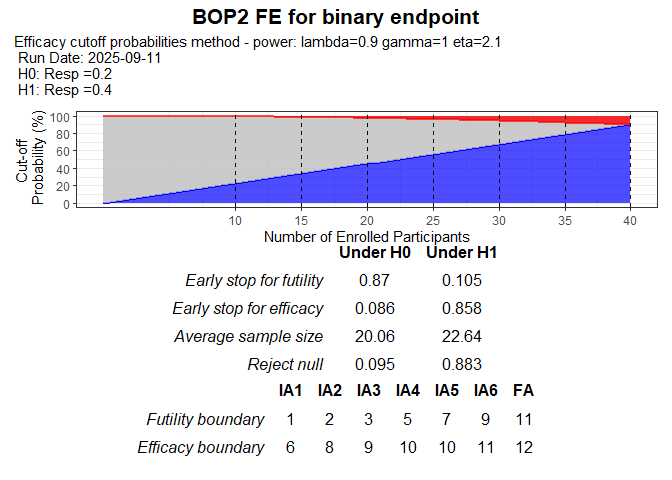
#> 1 0.9 1 2.1
#>
#> $boundary
#> IA1 IA2 IA3 IA4 IA5 IA6 FA
#> Futility boundary 1 2 3 5 7 9 11
#> Efficacy boundary 6 8 9 10 10 11 12
#>
#> $oc
#> Under H0 Under H1
#> Early stop for futility 0.870 0.105
#> Early stop for efficacy 0.086 0.858
#> Average sample size 20.060 22.640
#> Reject null 0.095 0.883
The result of BOP2-FE can be visualized as follow
plot(test_binary)
Nested endpoint
test_nested <- BOP2FE_nested(
 H0=c(0.15,0.15, 0.70), H1= c(0.25,0.25, 0.50),
 n = c(10, 5, 5, 5, 5, 5, 5),
 nsim = 1000, t1e = 0.1, method = "power",
 lambda1 = 0, lambda2 = 1, grid1 = 11,
 gamma1 = 0, gamma2 = 1, grid2 = 11,
 eta1 = 0, eta2 = 3, grid3 = 31,
 seed = 123
)
summary(test_nested)
#> $design_pars
#> $design_pars$H0
#> [1] 0.15 0.15 0.70
#>
#> $design_pars$H1
#> [1] 0.25 0.25 0.50
#>
#> $design_pars$n
#> [1] 10  5  5  5  5  5  5
#>
#> $design_pars$cum_n
#> [1] 10 15 20 25 30 35 40
#>
#> $design_pars$nsim
#> [1] 1000
#>
#> $design_pars$t1e
#> [1] 0.1
#>
#> $design_pars$method
#> [1] "power"
#>
#>
#> $opt_pars
#>   lambda gamma eta
#> 1    0.9   0.3   2
#>
#> $boundary
#>                           IA1 IA2 IA3 IA4 IA5 IA6 FA
#> Futility boundary (CR)      1   3   4   5   6   7  9
#> Futility boundary (CR/PR)   3   5   7   9  11  13 15
#> Efficacy boundary (CR)      6   6   7   8   9   9 10
#> Efficacy boundary (CR/PR)   8   9  11  12  14  15 16
#>
#> $oc
#>                         Under H0 Under H1
#> Early stop for futility    0.887    0.219
#> Early stop for efficacy    0.088    0.763
#> Average sample size       15.915   19.415
#> Reject null                0.098    0.778
Co-primary endpoint
test_coprimary <- BOP2FE_coprimary(
 H0=c(0.05,0.05, 0.15, 0.75),
 H1= c(0.15,0.15, 0.20, 0.50),
 n = c(10, 5, 5, 5, 5, 5, 5),
 nsim = 1000, t1e = 0.1, method = "power",
 lambda1 = 0, lambda2 = 1, grid1 = 11,
 gamma1 = 0, gamma2 = 1, grid2 = 11,
 eta1 = 0, eta2 = 3, grid3 = 31,
 seed = 123
)
summary(test_coprimary)
#> $design_pars
#> $design_pars$H0
#> [1] 0.05 0.05 0.15 0.75
#>
#> $design_pars$H1
#> [1] 0.15 0.15 0.20 0.50
#>
#> $design_pars$n
#> [1] 10  5  5  5  5  5  5
#>
#> $design_pars$cum_n
#> [1] 10 15 20 25 30 35 40
#>
#> $design_pars$nsim
#> [1] 1000
#>
#> $design_pars$t1e
#> [1] 0.1
#>
#> $design_pars$method
#> [1] "power"
#>
#>
#> $opt_pars
#>   lambda gamma eta
#> 1    0.9   0.3 2.3
#>
#> $boundary
#>                          IA1 IA2 IA3 IA4 IA5 IA6 FA
#> Futility boundary (OR)     1   2   3   4   4   5  6
#> Futility boundary (PFS6)   2   3   5   6   8   9 11
#> Efficacy boundary (OR)     5   6   6   6   7   7  7
#> Efficacy boundary (PFS6)   7   8   9  10  11  11 12
#>
#> $oc
#>                         Under H0 Under H1
#> Early stop for futility    0.880    0.096
#> Early stop for efficacy    0.084    0.899
#> Average sample size       16.285   18.710
#> Reject null                0.098    0.902
#plot(test_coprimary)
Joint endpoint
test_joint <- BOP2FE_jointefftox(
 H0=c(0.15,0.30, 0.15, 0.40),
 H1= c(0.18,0.42, 0.02, 0.38),
 n = c(10, 5, 5, 5, 5, 5, 5),
 nsim = 1000, t1e = 0.1, method = "power",
 lambda1 = 0, lambda2 = 1, grid1 = 11,
 gamma1 = 0, gamma2 = 1, grid2 = 11,
 eta1 = 0, eta2 = 3, grid3 = 31,
 seed = 123
)
summary(test_joint)
#> $design_pars
#> $design_pars$H0
#> [1] 0.15 0.30 0.15 0.40
#>
#> $design_pars$H1
#> [1] 0.18 0.42 0.02 0.38
#>
#> $design_pars$n
#> [1] 10  5  5  5  5  5  5
#>
#> $design_pars$cum_n
#> [1] 10 15 20 25 30 35 40
#>
#> $design_pars$nsim
#> [1] 1000
#>
#> $design_pars$t1e
#> [1] 0.1
#>
#> $design_pars$method
#> [1] "power"
#>
#>
#> $opt_pars
#>   lambda gamma eta
#> 1    0.7   0.8 0.9
#>
#> $boundary
#>                         IA1 IA2 IA3 IA4 IA5 IA6 FA
#> Futility boundary (OR)    3   5   8  11  13  16 19
#> Futility boundary (Tox)   5   6   7   8   9  10 11
#> Efficacy boundary (OR)    7  10  12  14  16  18 20
#> Efficacy boundary (Tox)   1   2   4   5   7   8 10
#>
#> $oc
#>                         Under H0 Under H1
#> Early stop for futility    0.886    0.311
#> Early stop for efficacy    0.094    0.646
#> Average sample size       18.020   22.085
#> Reject null                0.099    0.676
#plot(test_joint)