Description
Visualizing the Elements Within Bio-Sequences.
Description
Visualizing the types and distribution of elements within bio-sequences. At the same time, We have developed a geom layer, geom_rrect(), that can generate rounded rectangles. No external references are used in the development of this package.
README.md
BioVizSeq
1. Introduction
The goal of BioVizSeq is to visualize the types and distribution of elements within bio-sequences. At the same time, We have developed a geom layer, geom_rrect(), that can generate rounded rectangles. No external references are used in the development of this package.
2. Installation
Install from CRAN:
# Install from CRAN
install.packages("BioVizSeq")
Install from Github: the development version of BioVizSeq:
install.packages("devtools")
devtools::install_github("zhaosq2022/BioVizSeq")
3. Libary packages
library(BioVizSeq)
#> Registered S3 methods overwritten by 'treeio':
#>   method              from
#>   MRCA.phylo          tidytree
#>   MRCA.treedata       tidytree
#>   Nnode.treedata      tidytree
#>   Ntip.treedata       tidytree
#>   ancestor.phylo      tidytree
#>   ancestor.treedata   tidytree
#>   child.phylo         tidytree
#>   child.treedata      tidytree
#>   full_join.phylo     tidytree
#>   full_join.treedata  tidytree
#>   groupClade.phylo    tidytree
#>   groupClade.treedata tidytree
#>   groupOTU.phylo      tidytree
#>   groupOTU.treedata   tidytree
#>   inner_join.phylo    tidytree
#>   inner_join.treedata tidytree
#>   is.rooted.treedata  tidytree
#>   nodeid.phylo        tidytree
#>   nodeid.treedata     tidytree
#>   nodelab.phylo       tidytree
#>   nodelab.treedata    tidytree
#>   offspring.phylo     tidytree
#>   offspring.treedata  tidytree
#>   parent.phylo        tidytree
#>   parent.treedata     tidytree
#>   root.treedata       tidytree
#>   rootnode.phylo      tidytree
#>   sibling.phylo       tidytree
#> Package BioVizSeq loaded successfully!

# Extra package
library(ggplot2)
#> Warning: 程辑包'ggplot2'是用R版本4.3.3 来建造的
4. Usage cases
4.1 GFF/GTF
gff or gtf file
4.1.1 Step by step
gff_path <- system.file("extdata", "idpro.gff3", package = "BioVizSeq")
gff_data <- read.table(gff_path, header = FALSE, sep = '\t')
gff_loc <- gff_to_loc(gff_data)
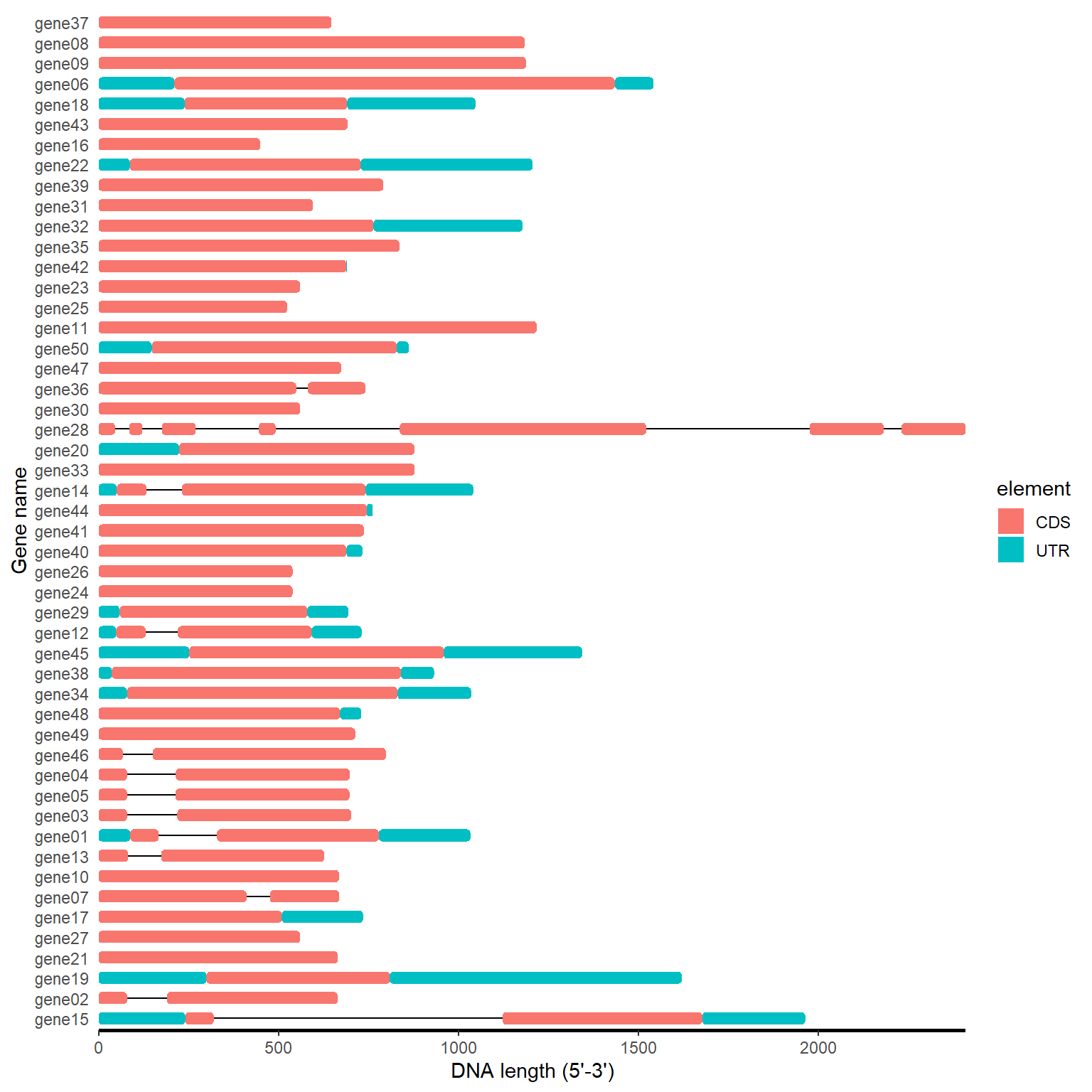
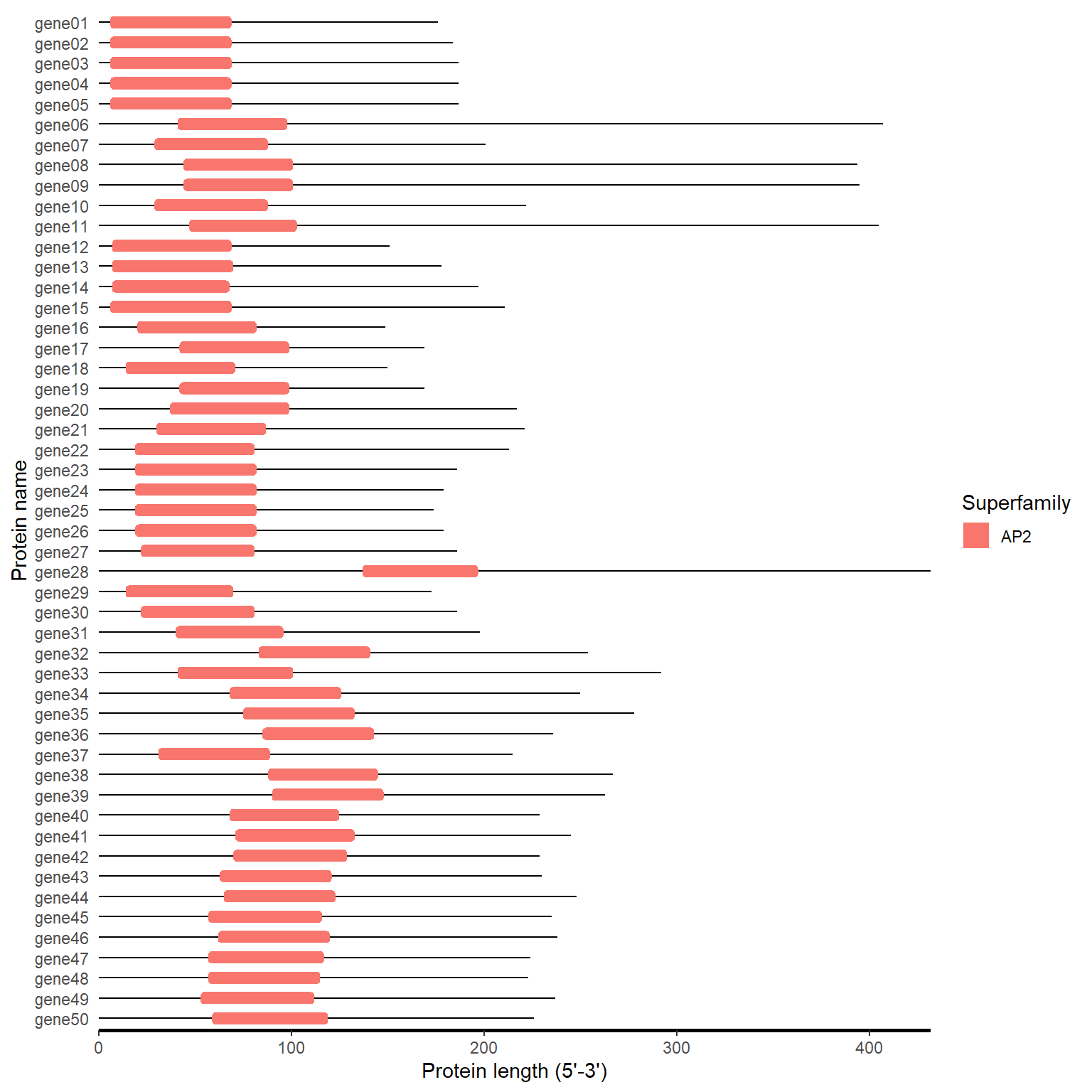
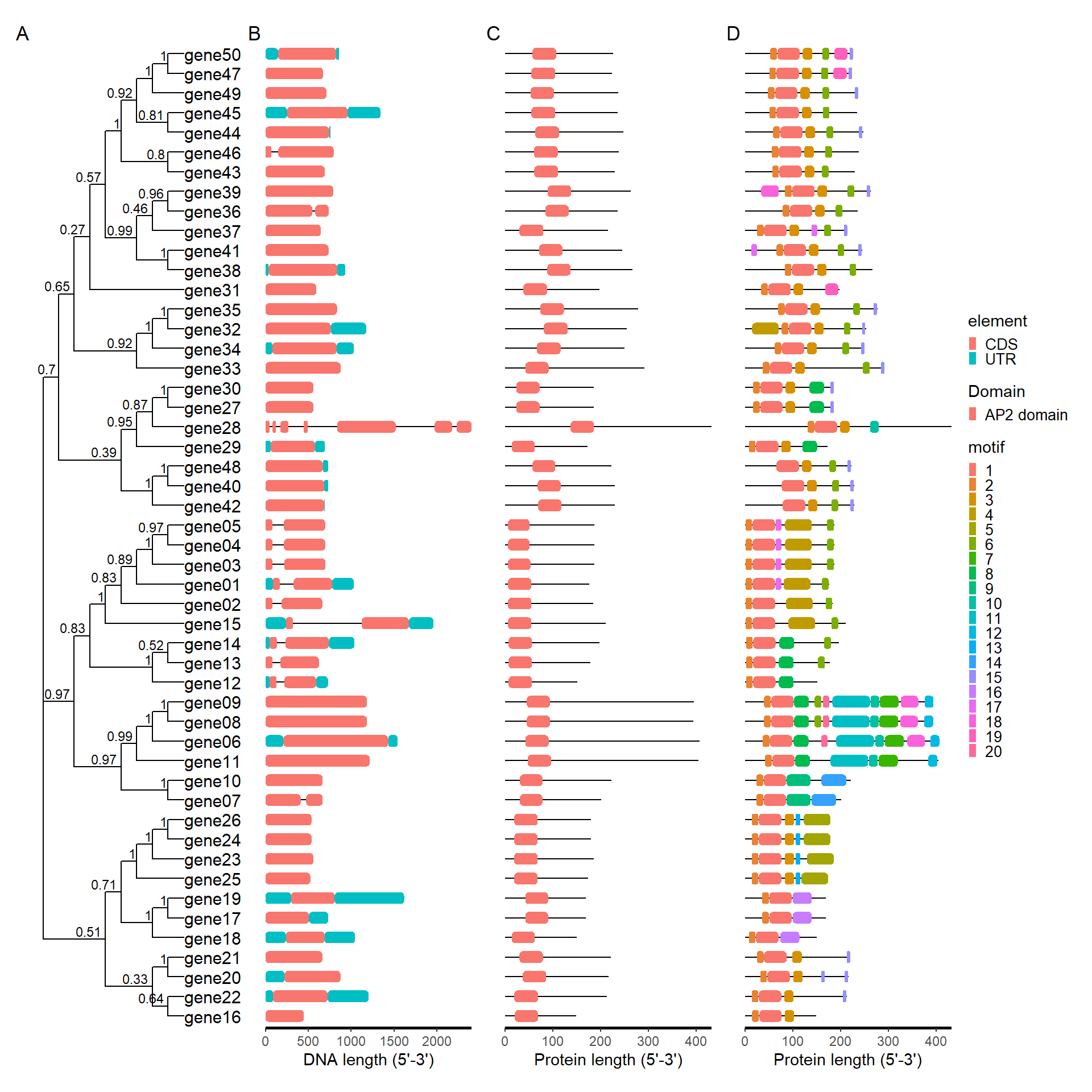
motif_plot(gff_loc$table_loc, gff_loc$gene_length) +
labs(x="DNA length (5'-3')", y="Gene name")
4.1.2 One step
gff_path <- system.file("extdata", "idpro.gff3", package = "BioVizSeq")
gff_plot(gff_path)

4.2 MEME
meme.xml or mast.xml
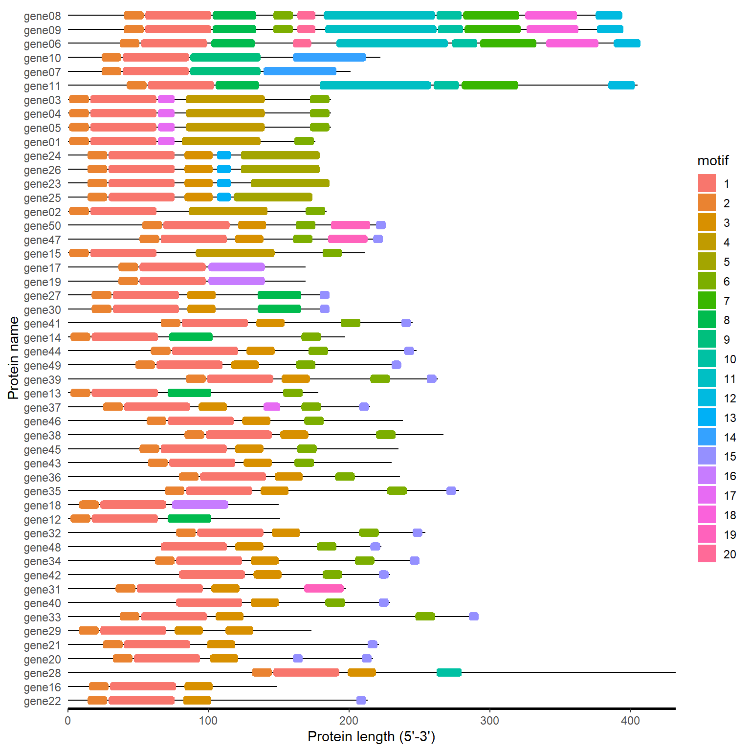
4.2.1 Step by step
meme_path <- system.file("extdata", "mast.xml", package = "BioVizSeq")
meme_file <- readLines(meme_path)
motif_loc <- meme_to_loc(meme_file)

motif_plot(motif_loc$table_loc, motif_loc$gene_length)
4.2.2 One step
meme_path <- system.file("extdata", "mast.xml", package = "BioVizSeq")
meme_plot(meme_path)
4.3 PFAM
Download: .tsv
4.3.1 Step by step
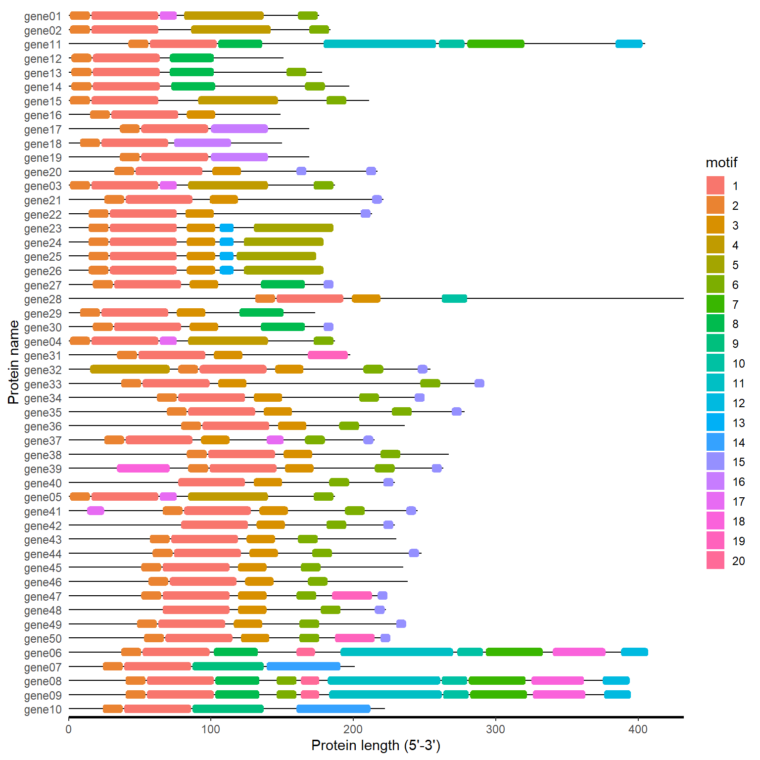
pfam_path <- system.file("extdata", "iprscan.tsv", package = "BioVizSeq")
pfam_file <- read.table(pfam_path, sep='\t', header = FALSE)
domain_loc <- pfam_to_loc(pfam_file)

motif_plot(domain_loc$table_loc, domain_loc$gene_length)
4.3.2 One step
pfam_path <- system.file("extdata", "iprscan.tsv", package = "BioVizSeq")
pfam_plot(pfam_path)

4.4 CDD
Download “Superfamily Only”
Type: .txt
4.4.1 Step by step
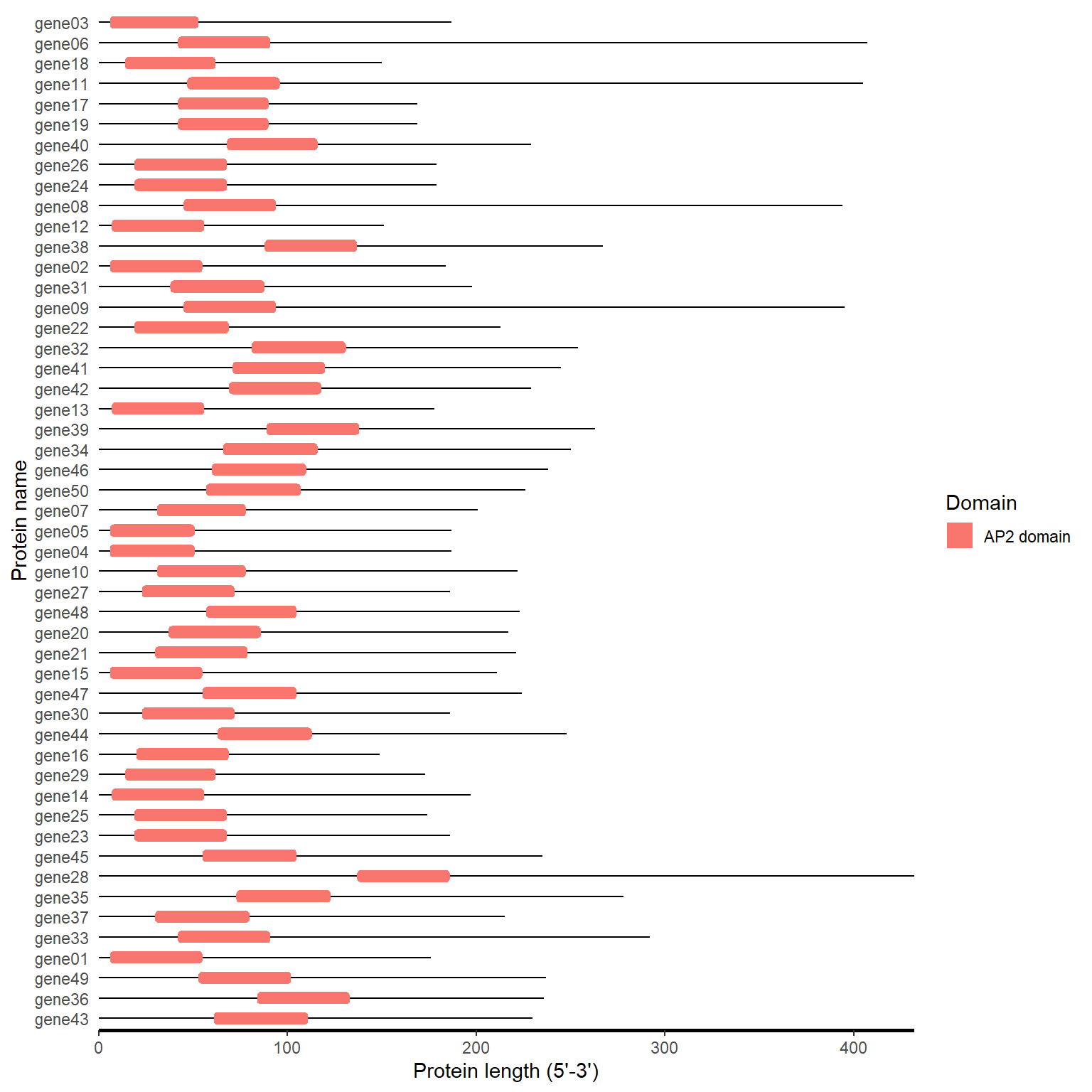
hitdata_path <- system.file("extdata", "hitdata.txt", package = "BioVizSeq")
cdd_file <- readLines(hitdata_path)
domain_loc <- cdd_to_loc(cdd_file)

fa_path <- system.file("extdata", "idpep.fa", package = "BioVizSeq")
gene_length <- fastaleng(fa_path)
motif_plot(domain_loc, gene_length)

4.4.2 One step
hitdata_path <- system.file("extdata", "hitdata.txt", package = "BioVizSeq")
fa_path <- system.file("extdata", "idpep.fa", package = "BioVizSeq")

cdd_plot(hitdata_path, fa_path)
4.5 SMART
protein file (.fa or .fasta)
4.5.1 Step by step
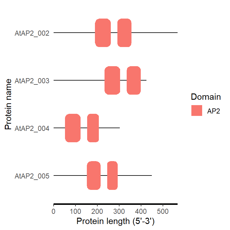
fa_path <- system.file("extdata", "target.fa", package = "BioVizSeq")
domain_loc <- smart_to_loc(fa_path)
#> Submitting sequence AtAP2_002...
#> Submitting sequence AtAP2_003...
#> Job entered the queue with ID12315310532459281744966748fjuQJesKfo. Waiting for results.
#> Submitting sequence AtAP2_004...
#> Submitting sequence AtAP2_005...

motif_plot(domain_loc$table_loc, domain_loc$gene_length)

4.5.2 One step
fa_path <- system.file("extdata", "target.fa", package = "BioVizSeq")

smart_plot(fa_path)
#> Submitting sequence AtAP2_002...
#> Submitting sequence AtAP2_003...
#> Job entered the queue with ID12315310532468761744966784YObRQLBBcV. Waiting for results.
#> Submitting sequence AtAP2_004...
#> Submitting sequence AtAP2_005...
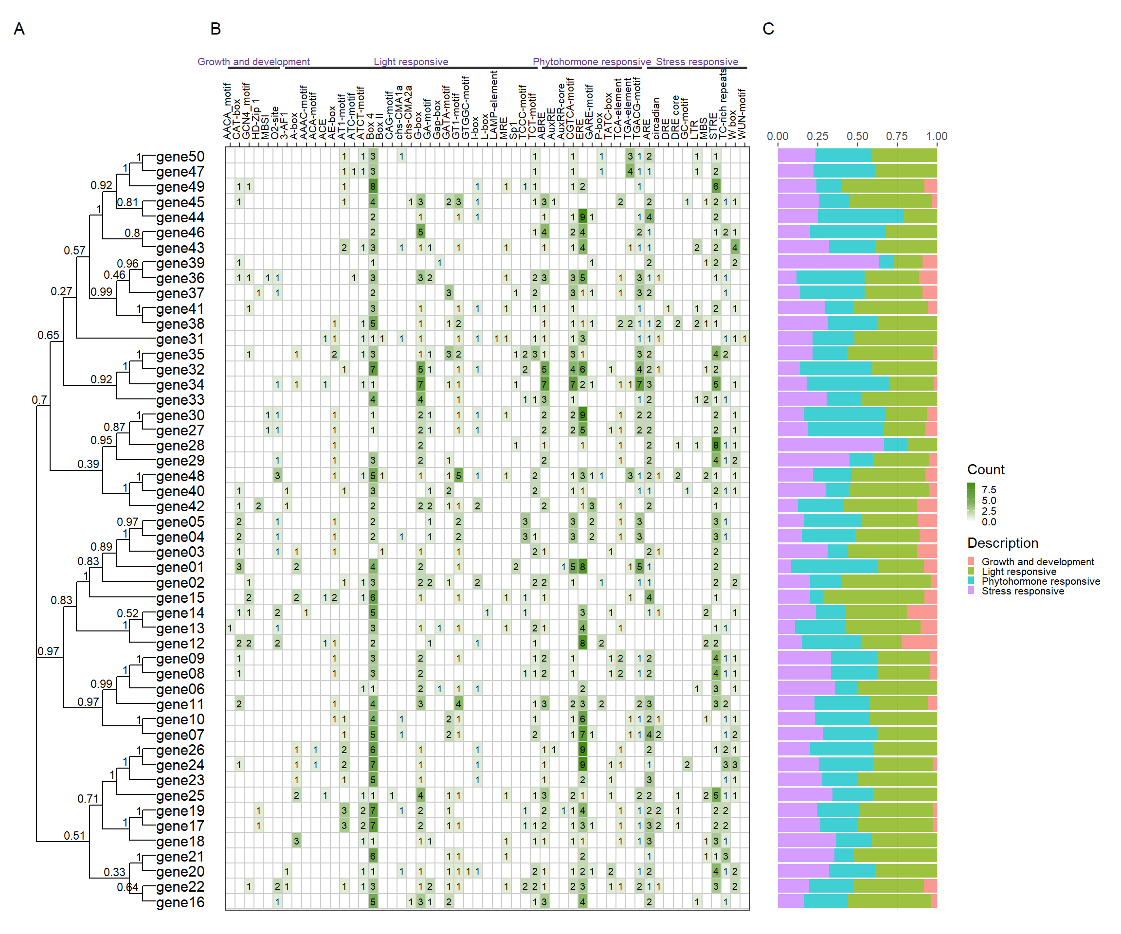
4.6 Plantcare
promoter sequence(.fa or .fasta)
4.6.1 Step by step
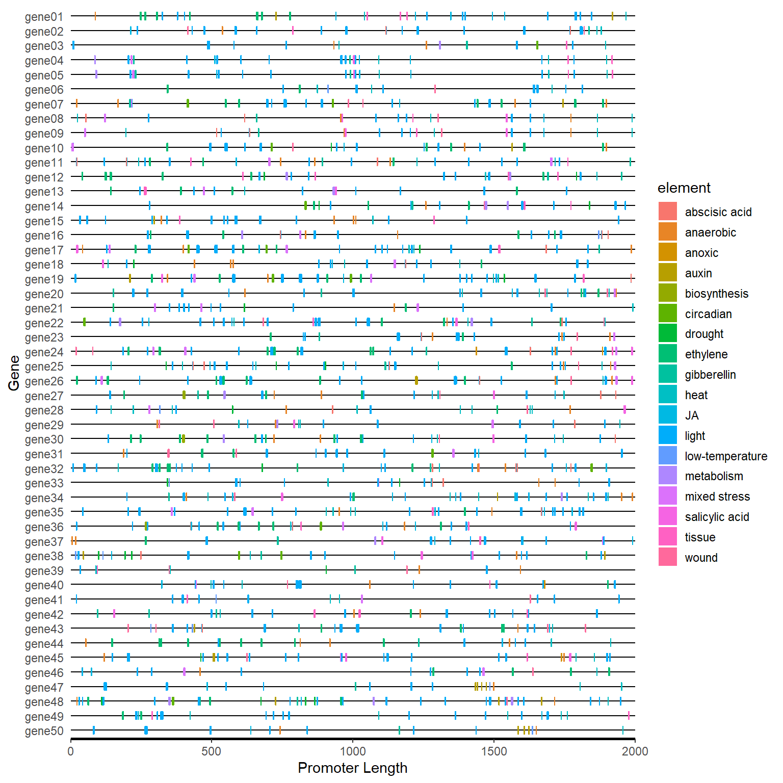
# 1. upload fasta file to plantcare, get the result file(.tab)
# upload_fa_to_plantcare(fasta_file, email)

# 2. Classify the functions of cis element

plantcare_path <- system.file("extdata", "plantCARE_output.tab", package = "BioVizSeq")
plantcare_file <- read.table(plantcare_path, header = FALSE, sep = '\t', quote="")
plantcare_data <- plantcare_classify(plantcare_file)
plantcare_loc <- plantcare_to_loc(plantcare_data)

promoter_length <- data.frame(ID = unique(plantcare_loc$ID), length=2000)

motif_plot(plantcare_loc, promoter_length) +
    labs(x="Promoter Length", y="Gene")
4.6.2 One step
plantcare_path <- system.file("extdata", "plantCARE_output.tab", package = "BioVizSeq")
plantcare_plot(plantcare_path, promoter_length = 2000)
4.7 Advance Plot
p_tree, p_gff, p_pfam, p_meme, p_smart, p_cdd, p_plantcare
library(patchwork)
tree_path <- system.file("extdata", "idpep.nwk", package = "BioVizSeq")
gff_path <- system.file("extdata", "idpro.gff3", package = "BioVizSeq")
meme_path <- system.file("extdata", "mast.xml", package = "BioVizSeq")
pfam_path <- system.file("extdata", "iprscan.tsv", package = "BioVizSeq")
plot_file <- combi_p(tree_path = tree_path, gff_path = gff_path,
                     meme_path = meme_path, pfam_path = pfam_path)

plot_file$p_tree + plot_file$p_gff + plot_file$p_pfam +
  plot_file$p_meme +plot_layout(ncol = 4, guides = 'collect') +
  plot_annotation(
    tag_levels = 'A'
  )
library(patchwork)
tree_path <- system.file("extdata", "idpep.nwk", package = "BioVizSeq")
plantcare_path <- system.file("extdata", "plantCARE_output.tab", package = "BioVizSeq")
plot_file <- combi_p(tree_path = tree_path, plantcare_path = plantcare_path, promoter_length = 2000)

plot_file$p_tree + plot_file$p_plantcare1 + plot_file$p_plantcare2 + plot_layout(ncol = 3, guides = 'collect', widths = c(1, 3, 1)) + plot_annotation( tag_levels = 'A' )
4.8 Gene and Protein calc
gff_path <- system.file("extdata", "idpro.gff3", package = "BioVizSeq")
gff_data <- read.table(gff_path, header = FALSE, sep = '\t')
gene_statistics_data <- gff_statistics(gff_data)
head(gene_statistics_data)
#>       ID                Location Chain gene_length CDS_length protein_length
#> 1 gene01 Chr15:31085288-31086321     -        1034        531            176
#> 2 gene02   Contig862:15967-16631     -         665        555            184
#> 3 gene03 Chr15:31004816-31005518     +         703        564            187
#> 4 gene04 Chr15:30780257-30780955     +         699        564            187
#> 5 gene05 Chr15:30976079-30976776     +         698        564            187
#> 6 gene06  Chr2:12719447-12720989     +        1543       1224            407
#>   exon_number intron_number CDS_number UTR_number
#> 1           2             1          2          2
#> 2           2             1          2          0
#> 3           2             1          2          0
#> 4           2             1          2          0
#> 5           2             1          2          0
#> 6           1             0          1          2

pep_path <- system.file("extdata", "idpep2.fa", package = "BioVizSeq")
pep_calc_result <- ProtParam_calc(pep_path)
#> Submitting sequence gene01...
#> Submitting sequence gene02...
#> Submitting sequence gene03...
head(pep_calc_result)
#>       ID Number of amino acids Molecular weight Theoretical pI
#> 1 gene01                   176         19433.92           6.22
#> 2 gene02                   184         20288.83           9.07
#> 3 gene03                   187         21042.90           7.68
#>   The instability index Aliphatic index Grand average of hydropathicity
#> 1                 80.30           67.16                          -0.611
#> 2                 68.69           73.15                          -0.580
#> 3                 72.86           69.41                          -0.637