Cumulative Odds Ratio Plot.
README
CORPlot
The goal of CORPlot is to create cumulative odds ratio plot to visually inspect the proportional odds assumption from the proportional odds model. For more explanation on the role of the proportional odds assumption in ordinal outcome analysis, see our paper (Long et. al, 2025).
Installation
You can install the development version of CORPlot from GitHub with:
# install.packages("pak")
pak::pak("Yongxi-Long/CORPlot")
Example
There are three steps to make a cumulative odds ratio plot, each corresponds to a function in this package:
- PerformLogReg(): Perform cumulative logistic regression (i.e., no proportionality constraint) and get all binary odds ratios
- PerformPO(): Perform the proportional odds model and get the common odds ratio
- CORPlot(): Create the cumulative odds ratio plot
Users can either directly input to the CORPlot() funtion and this function will do the first two steps internally. Or users can choose to supplied a data frame of odds ratios calculated externally and ask CORPlot to make the plot.
The dataset
We will use the df_MR_CLEAN example dataset included in the package. It is from a randomized controlled trial investigating endovascular therapy in patients with stroke (Berkhemer et al., 2015). The trial enrolled 500 patients, with 233 assigned to the intervention group and 267 to the control group. The dataset contains three variables:
- mRS: Modified Rankin Scale. A 7-point ordinal scale used to measure patient outcomes
- group: Group assignment. 1 = Intervention, 0 = Control
- sex: Simulated variable for sex. 1 = Women, 0 = Men
Because very few patients fell into mRS category 0, we combine categories 0 and 1 into a single category (labeled mRS = 1) to improve representation in the Cumulative Odds Ratio plot.
data("df_MR_CLEAN")
df_MR_CLEAN <- df_MR_CLEAN |>
  dplyr::mutate(mRS6 = dplyr::case_when(
    mRS <= 1 ~ 1,
    TRUE ~ mRS
  ))
Use CORPlot() directly
res <- CORPlot(
data = df_MR_CLEAN,
formula = mRS6 ~ group,
GroupName = "group",
confLevel = 0.9
)
# show the plot
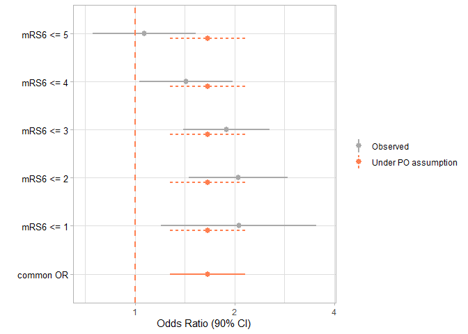
plot(res)
# print the detailed ORs and confidence intervals
print(res,digits = 3)
#>
#>
#> Table: Odds Ratios
#>
#> |   Label   |  OR   | lowerCI | upperCI |   type   |
#> |:---------:|:-----:|:-------:|:-------:|:--------:|
#> | mRS6 <= 1 | 2.056 |  1.196  |  3.534  | Observed |
#> | mRS6 <= 2 | 2.050 |  1.453  |  2.892  | Observed |
#> | mRS6 <= 3 | 1.890 |  1.399  |  2.554  | Observed |
#> | mRS6 <= 4 | 1.426 |  1.032  |  1.970  | Observed |
#> | mRS6 <= 5 | 1.065 |  0.744  |  1.525  | Observed |
#> | common OR | 1.657 |  1.274  |  2.155  | Observed |
Step-by-step construction
We can also calculate the binary odds ratios and the common odds ratio from elsewhere and supply a data.frame to CORPlot() to make the plot only. The input data.frame must have the following columns:
- Label: label to distinguish the binary odds ratios for different cutpoints and the common odds ratio
- There must be a label identifying the common odds ratio, can be one of “common odds ratio”, “common OR”, “cOR” (case insensitive).
- OR: odds ratios
- lowerCI: lower bound for the confidence interval
- upperCI: upper bound for the confidence interval
## use PerforLogReg function to get all binary odds ratios
# We calculate the odds ratio for the group effect, adjusted by sex
# This is done by putting both group and sex in the formula
# and ask for group effect by letting GroupName = "group"
# similarly, if we want the odds ratio of the sex effect, adjusted by group
# we can let GroupName = "sex"

binary_ORs_df <- PerformLogReg(data=df_MR_CLEAN,
              formula = mRS6~group+sex,
              GroupName = "group",
              upper = FALSE)

## use PerformPO to get the common odds ratio
cOR_df <- PerformPO(data=df_MR_CLEAN,
              formula = mRS6~group+sex,
              GroupName = "group",
              upper = FALSE)

## Combine the data.frame
OR_df <- rbind(binary_ORs_df,
               cOR_df)
OR_df |>
  kable(digits = 3, format = "markdown",
        caption = "Binary odds ratios and common odds ratio of the 7-point mRS outcome in the MR CLEAN trial")
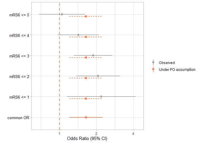
| Label | OR | lowerCI | upperCI |
|---|---|---|---|
| mRS6 <= 1 | 2.195 | 1.154 | 4.175 |
| mRS6 <= 2 | 2.063 | 1.369 | 3.110 |
| mRS6 <= 3 | 1.878 | 1.312 | 2.690 |
| mRS6 <= 4 | 1.425 | 0.968 | 2.096 |
| mRS6 <= 5 | 1.049 | 0.684 | 1.608 |
| common OR | 1.647 | 1.204 | 2.253 |
Binary odds ratios and common odds ratio of the 7-point mRS outcome in the MR CLEAN trial
## Feed this data.frame to the CORPlot function
res2 <- CORPlot(OR_df = OR_df)
plot(res2)
Reference
Berkhemer, O. A., Fransen, P. S., Beumer, D., Van Den Berg, L. A., Lingsma, H. F., Yoo, A. J., et al.others. (2015). A randomized trial of intraarterial treatment for acute ischemic stroke. New England Journal of Medicine, 372(1), 11–20.
Long, Y., Wiegers, E. J. A., Jacobs, B. C., Steyerberg, E. W., & Van Zwet, E. W. (2025). Role of the Proportional Odds Assumption for the Analysis of Ordinal Outcomes in Neurologic Trials. Neurology, 105(8), e214146.