Identify Changes in Mean.
ChangePointTaylor
The goal of ChangePointTaylor is to identify changes in mean for a series of data. The package is a simple R implementation of the change in mean detection method developed by Wayne Taylor and utilized in his Change Point Analyzer software. The package recursively uses the ‘MSE’ change point calculation to identify candidate change points. The change points are then re-estimated and Taylor’s backwards elimination process is employed to come up with a final set of change points. Many of the underlying functions are written in C++ for improved performance.
Installation
You can install the released version of ChangePointTaylor from CRAN with:
install.packages("ChangePointTaylor")
Example
Load the package and tidyverse.
library(ChangePointTaylor)
library(tidyverse)
#> -- Attaching packages ------------------------------------------------------------------------------------------------------------------------- tidyverse 1.3.0 --
#> v ggplot2 3.3.0     v purrr   0.3.4
#> v tibble  3.0.1     v dplyr   0.8.5
#> v tidyr   1.0.3     v stringr 1.4.0
#> v readr   1.3.1     v forcats 0.5.0
#> -- Conflicts ---------------------------------------------------------------------------------------------------------------------------- tidyverse_conflicts() --
#> x dplyr::filter() masks stats::filter()
#> x dplyr::lag()    masks stats::lag()
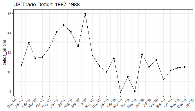
View the example dataset of US trade deficit data from January 1987 to December 1988.
US_Trade_Deficit
#> # A tibble: 24 x 2
#>    date    deficit_billions
#>    <chr>              <dbl>
#>  1 Jan '87             10.7
#>  2 Feb '87             13
#>  3 Mar '87             11.4
#>  4 Apr '87             11.5
#>  5 May '87             12.5
#>  6 Jun '87             14.1
#>  7 Jul '87             14.8
#>  8 Aug '87             14.1
#>  9 Sep '87             12.6
#> 10 Oct '87             16
#> # ... with 14 more rows
Plot the data
trade_deficit_plot <- US_Trade_Deficit %>%
  mutate(date = as.Date(paste(date, "1"), format = "%b '%y %d")) %>%
  ggplot(aes(x = date, y = deficit_billions, group = 1)) +
  geom_line() +
  geom_point() +
  theme_bw() +
  scale_x_date(date_breaks = "1 month", date_labels = "%b '%y") +
  theme(
    axis.text.x = element_text(angle = 45, vjust = 1, hjust =1),
    axis.title.x = element_blank()
  ) +
  ggtitle("US Trade Deficit: 1987-1988")

trade_deficit_plot

In its simplest form, the change_point_analyzer() function simply takes a numeric vector and returns the identified change points. However, the output only identifies changes by their index in the original numeric vector.
change_point_analyzer(US_Trade_Deficit$deficit_billions)
#> 2 Change(s) Identified
#> NA supplied to 'label' argument
#> # A tibble: 2 x 6
#>   change_ix label `CI (95%)` change_conf  From    To
#>       <dbl> <lgl> <chr>            <dbl> <dbl> <dbl>
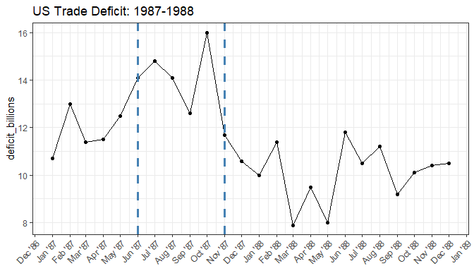
#> 1         6 NA    (5 - 7)          0.938  11.8  14.3
#> 2        11 NA    (11 - 11)        0.999  14.3  10.2
When a vector of labels, the same length as the x values, is supplied to the label argument, those labels will be displayed in the output dataframe.
change_points <- change_point_analyzer(US_Trade_Deficit$deficit_billions, label = US_Trade_Deficit$date)
#> 2 Change(s) Identified
change_points
#>   change_ix   label            CI (95%) change_conf  From    To
#> 1         6 Jun '87 (May '87 - Jul '87)       0.913 11.82 14.32
#> 2        11 Nov '87 (Nov '87 - Nov '87)       0.998 14.32 10.20
Plot the change points we identified.
trade_deficit_plot +
  geom_vline(xintercept = as.Date(paste(change_points$label, "1"), format = "%b '%y %d"), color = "steelblue", linetype = "dashed", size = 1.3)

The number of bootstraps can be controlled with the n_bootstraps argument. This can reduce stochastic differences between subsequent function calls; however, this comes at the expense of execution speed.
bench::mark(
  change_point_analyzer(US_Trade_Deficit$deficit_billions, label = US_Trade_Deficit$date, n_bootstraps = 1000)
 ,change_point_analyzer(US_Trade_Deficit$deficit_billions, label = US_Trade_Deficit$date, n_bootstraps = 10000)
  ,check = F
 ,min_iterations = 2
 ,max_iterations = 5
) %>%
  mutate(expression = c("1000 Bootstraps", "10000 Bootstraps")) %>%
  select(expression:mem_alloc)
#> # A tibble: 2 x 5
#>   expression            min   median `itr/sec` mem_alloc
#>   <chr>            <bch:tm> <bch:tm>     <dbl> <bch:byt>
#> 1 1000 Bootstraps  295.69ms 304.81ms     3.28      134MB
#> 2 10000 Bootstraps    1.03s    1.05s     0.948     274MB
The the user can also adjust the minimum level of confidence a change point must reach to become an initial candidate (min_candidate_conf) and the minimum confidence to be included in the final table of change points (min_tbl_conf).
change_point_analyzer(US_Trade_Deficit$deficit_billions, label = US_Trade_Deficit$date, min_candidate_conf = 0.66,  min_tbl_conf = 0.95)
#> 1 Change(s) Identified
#>   change_ix   label            CI (95%) change_conf     From       To
#> 1        12 Dec '87 (Sep '87 - Jan '88)           1 12.94545 10.08462