Description

Detecting Epidemics using School Absenteeism.

Description

Provides a comprehensive framework for early epidemic detection through school absenteeism surveillance. The package offers three core functionalities: (1) simulation of population structures, epidemic spread, and resulting school absenteeism patterns; (2) implementation of surveillance models that generate alerts for impending epidemics based on absenteeism data and (3) evaluation of alert timeliness and accuracy through alert time quality metrics to optimize model parameters. These tools enable public health officials and researchers to develop and assess early warning systems before implementation. Methods are based on research published in Vanderkruk et al. (2023) <doi:10.1186/s12889-023-15747-z> and Ward et al. (2019) <doi:10.1186/s12889-019-7521-7>.

README.md

cran.r-project.org

DESA: Detecting Epidemics using School Absenteeism <badges go here>

Overview

DESA provides a comprehensive framework for early epidemic detection through school absenteeism surveillance. The package enables:

Simulation: Generate realistic populations, epidemic spread patterns, and resulting school absenteeism data
Detection: Implement surveillance models that raise timely alerts for impending epidemics
Evaluation: Assess and optimize detection models using metrics that balance timeliness and accuracy

The methods implemented are based on research by Vanderkruk et al. (2023) and Ward et al. (2019).

Why School Absenteeism?

Children typically have higher influenza infection rates than other age groups and are encouraged to stay home when ill. This makes school absenteeism data a valuable early indicator of community-wide epidemic arrival, potentially providing public health officials with crucial lead time to implement mitigation strategies.

Background

Traditional epidemic surveillance systems often rely on laboratory-confirmed cases, which can introduce significant delays in detection. To address this limitation, Ward et al. (2019) investigated the use of school absenteeism data for early epidemic detection in the Wellington-Dufferin-Guelph region of Ontario, Canada.

The existing system in this region used a simple threshold-based approach (raising an alarm when 10% of students were absent) to identify potential outbreaks. Ward et al. developed detection models and introduced two evaluation metrics:

False Alert Rate (FAR): Measures the proportion of incorrectly raised alarms
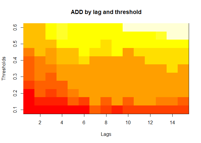
Accumulated Days Delayed (ADD): Quantifies the timeliness of correct alarms

Building on this foundation, Vanderkruk et al. (2023) developed a more nuanced evaluation framework called Alert Time Quality (ATQ). Unlike the binary classification of previous metrics, ATQ assesses alerts where ones that are raised at sub optimal times receive penalties proportional to their deviation from the ideal alert time. This approach balances both accuracy and timeliness in a single metric.

The DESA package implements the methodologies from both papers, enabling users to:

Generate simulations of population structures based on regional census data
Apply various detection models to simulated epidemics
Evaluate model performance using FAR, ADD, and ATQ-based metrics

Installation:

You can install the development version of DESA from Github

#install.packages("devtools")
library(devtools)
install_github("vjoshy/DESA")

Key Functions

The ATQ package includes the following main functions:

catchment_sim()
- Simulates catchment area data
elementary_pop()
- Simulates elementary school populations
subpop_children()
- Simulates households with children
subpop_noChildren()
- Simulates households without children
simulate_households()
- Combines household simulations
ssir()
- Simulates epidemic using SSIR model
compile_epi()
- Compiles absenteeism data
eval_metrics()
- Evaluates alarm metrics
plot() and summary()
- Methods for visualizing and summarizing results

Additionally, the package implements S3 methods for generic functions:

plot() and summary()
- These methods are extended for objects returned by ssir() and eval_metrics()
- plot() provides visualizations of epidemic simulations and metric evaluations
- summary() offers concise summaries of the simulation results and metric assessments

These functions and methods work together to facilitate comprehensive epidemic simulation and evaluation of detection models

Please see example below:

# Load the DESA package
library(DESA)

set.seed(69420)

#Simulate number of elementary schools in each catchment
catch_df <- catchment_sim(16, 5, shape = 4.68, rate = 3.01)

# Simulate elementary school populations for each catchment area
elementary_df <- elementary_pop(catch_df, shape = 5.86, rate = 0.01)

# Simulate households with children
house_children <- subpop_children(elementary_df, n = 2,
                                  prop_parent_couple = 0.7,
                                  prop_children_couple = c(0.3, 0.5, 0.2),
                                  prop_children_lone = c(0.4, 0.4, 0.2),
                                  prop_elem_age = 0.6)

# Simulate households without children
house_nochildren <-  subpop_noChildren(house_children, elementary_df,
                                   prop_house_size = c(0.2, 0.3, 0.25, 0.15, 0.1),
                                   prop_house_Children = 0.3)

# Combine household simulations and generate individual-level data
simulation <- simulate_households(house_children, house_nochildren)

# Extract individual-level data
individuals <- simulation$individual_sim

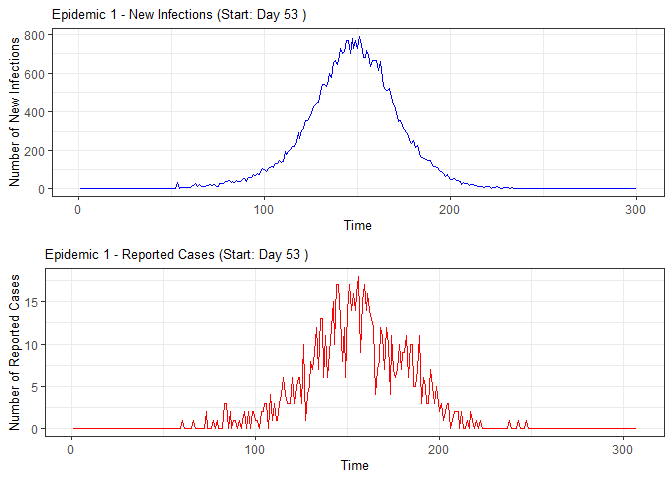
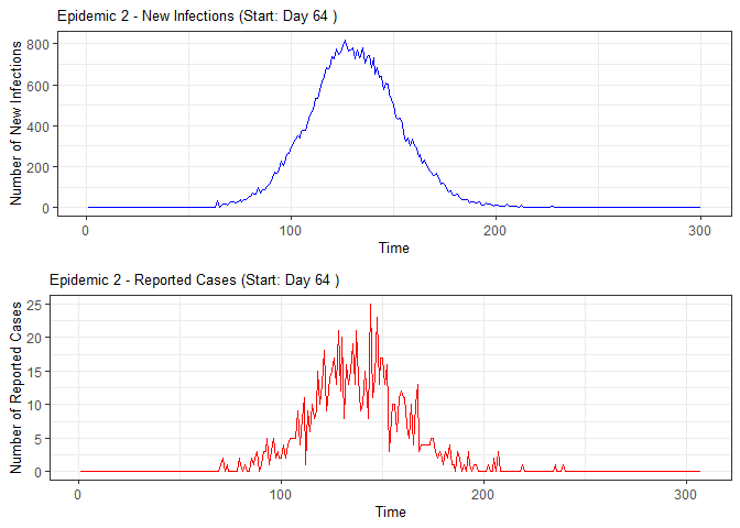
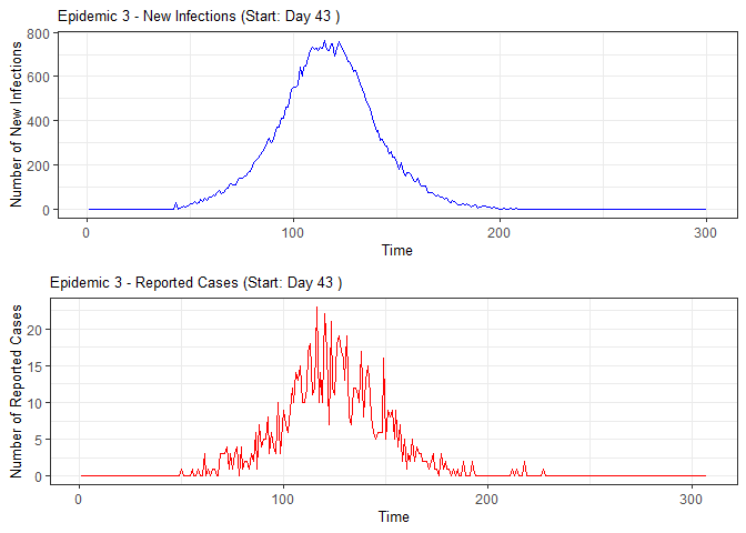
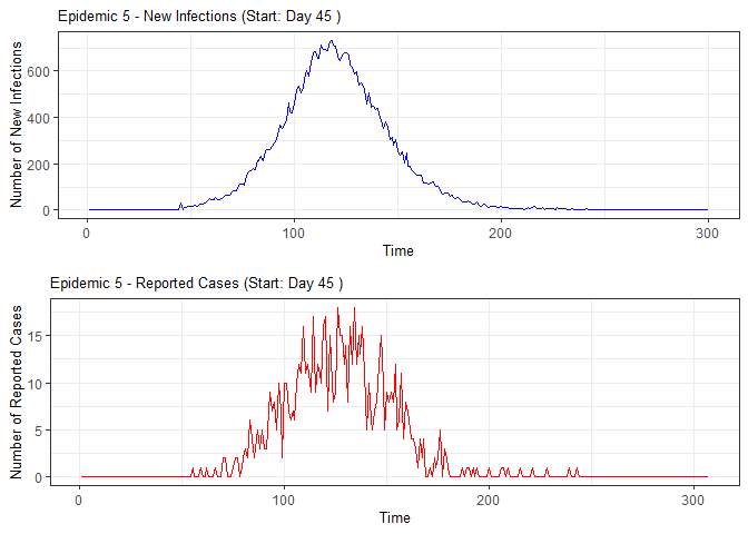
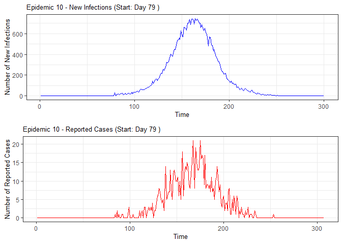
# Simulate epidemic using SSIR (Stochastic Susceptible-Infectious-Recovered) model
epidemic <- ssir(nrow(individuals), T = 300, alpha = 0.298, inf_init = 32, rep = 10)

# Summarize and plot the epidemic simulation results
summary(epidemic)
#> SSIR Epidemic Summary (Multiple Simulations):
#> Number of simulations: 10 
#> 
#> Average total infected: 41065.5 
#> Average total reported cases: 826.9 
#> Average peak infected: 3036.4 
#> 
#> Model parameters:
#> $N
#> [1] 136784
#> 
#> $T
#> [1] 300
#> 
#> $alpha
#> [1] 0.298
#> 
#> $inf_period
#> [1] 4
#> 
#> $inf_init
#> [1] 32
#> 
#> $report
#> [1] 0.02
#> 
#> $lag
#> [1] 7
#> 
#> $rep
#> [1] 10
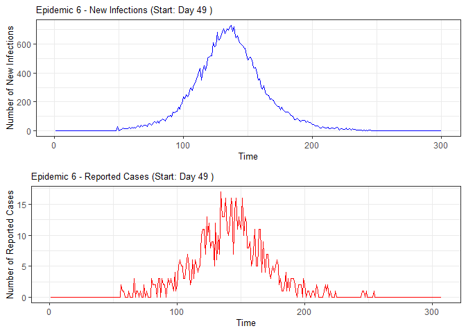
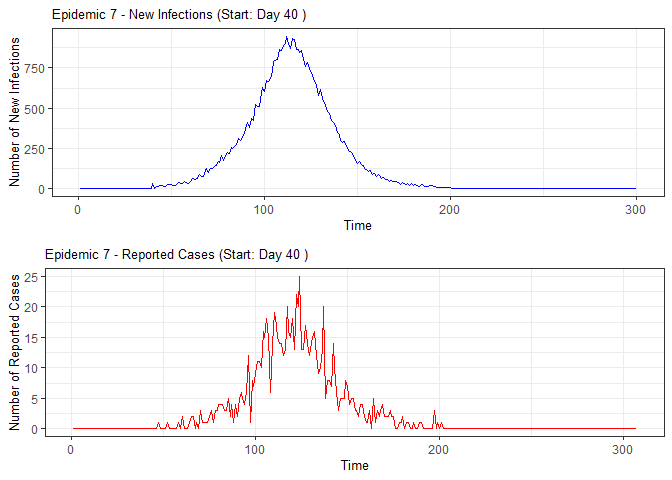
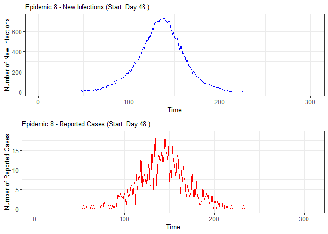
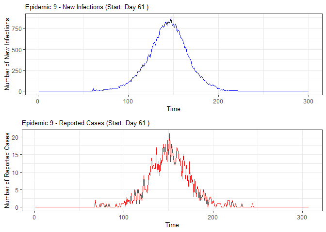
plot(epidemic)


# Compile absenteeism data based on epidemic simulation and individual data
absent_data <- compile_epi(epidemic, individuals)

# Display structure of absenteeism data
dplyr::glimpse(absent_data)
#> Rows: 3,000
#> Columns: 28
#> $ Date        <int> 1, 2, 3, 4, 5, 6, 7, 8, 9, 10, 11, 12, 13, 14, 15, 16, 17,…
#> $ ScYr        <int> 1, 1, 1, 1, 1, 1, 1, 1, 1, 1, 1, 1, 1, 1, 1, 1, 1, 1, 1, 1…
#> $ pct_absent  <dbl> 0.05096603, 0.05190044, 0.05079590, 0.04899765, 0.05083607…
#> $ absent      <dbl> 636, 661, 628, 627, 623, 624, 607, 603, 657, 673, 616, 667…
#> $ absent_sick <dbl> 0, 0, 0, 0, 0, 0, 0, 0, 0, 0, 0, 0, 0, 0, 0, 0, 0, 0, 0, 0…
#> $ new_inf     <dbl> 0, 0, 0, 0, 0, 0, 0, 0, 0, 0, 0, 0, 0, 0, 0, 0, 0, 0, 0, 0…
#> $ lab_conf    <dbl> 0, 0, 0, 0, 0, 0, 0, 0, 0, 0, 0, 0, 0, 0, 0, 0, 0, 0, 0, 0…
#> $ Case        <dbl> 0, 0, 0, 0, 0, 0, 0, 0, 0, 0, 0, 0, 0, 0, 0, 0, 0, 0, 0, 0…
#> $ sinterm     <dbl> 0.01720158, 0.03439806, 0.05158437, 0.06875541, 0.08590610…
#> $ costerm     <dbl> 0.9998520, 0.9994082, 0.9986686, 0.9976335, 0.9963032, 0.9…
#> $ window      <dbl> 0, 0, 0, 0, 0, 0, 0, 0, 0, 0, 0, 0, 0, 0, 0, 0, 0, 0, 0, 0…
#> $ ref_date    <dbl> 0, 0, 0, 0, 0, 0, 0, 0, 0, 0, 0, 0, 0, 0, 0, 0, 0, 0, 0, 0…
#> $ lag0        <dbl> 0.05096603, 0.05190044, 0.05079590, 0.04899765, 0.05083607…
#> $ lag1        <dbl> NA, 0.05096603, 0.05190044, 0.05079590, 0.04899765, 0.0508…
#> $ lag2        <dbl> NA, NA, 0.05096603, 0.05190044, 0.05079590, 0.04899765, 0.…
#> $ lag3        <dbl> NA, NA, NA, 0.05096603, 0.05190044, 0.05079590, 0.04899765…
#> $ lag4        <dbl> NA, NA, NA, NA, 0.05096603, 0.05190044, 0.05079590, 0.0489…
#> $ lag5        <dbl> NA, NA, NA, NA, NA, 0.05096603, 0.05190044, 0.05079590, 0.…
#> $ lag6        <dbl> NA, NA, NA, NA, NA, NA, 0.05096603, 0.05190044, 0.05079590…
#> $ lag7        <dbl> NA, NA, NA, NA, NA, NA, NA, 0.05096603, 0.05190044, 0.0507…
#> $ lag8        <dbl> NA, NA, NA, NA, NA, NA, NA, NA, 0.05096603, 0.05190044, 0.…
#> $ lag9        <dbl> NA, NA, NA, NA, NA, NA, NA, NA, NA, 0.05096603, 0.05190044…
#> $ lag10       <dbl> NA, NA, NA, NA, NA, NA, NA, NA, NA, NA, 0.05096603, 0.0519…
#> $ lag11       <dbl> NA, NA, NA, NA, NA, NA, NA, NA, NA, NA, NA, 0.05096603, 0.…
#> $ lag12       <dbl> NA, NA, NA, NA, NA, NA, NA, NA, NA, NA, NA, NA, 0.05096603…
#> $ lag13       <dbl> NA, NA, NA, NA, NA, NA, NA, NA, NA, NA, NA, NA, NA, 0.0509…
#> $ lag14       <dbl> NA, NA, NA, NA, NA, NA, NA, NA, NA, NA, NA, NA, NA, NA, 0.…
#> $ lag15       <dbl> NA, NA, NA, NA, NA, NA, NA, NA, NA, NA, NA, NA, NA, NA, NA…

# Evaluate alarm metrics for epidemic detection
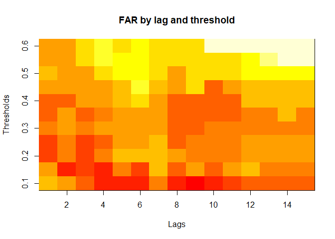
alarm_metrics <- eval_metrics(absent_data, thres = seq(0.1,0.6,by = 0.05))

# Plot various alarm metrics
plot(alarm_metrics$metrics, "FAR")   # False Alert Rate

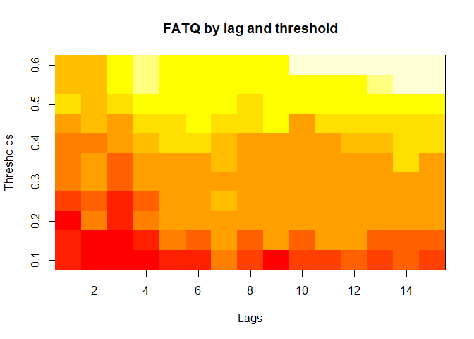
plot(alarm_metrics$metrics, "FATQ")  # First Alert Time Quality

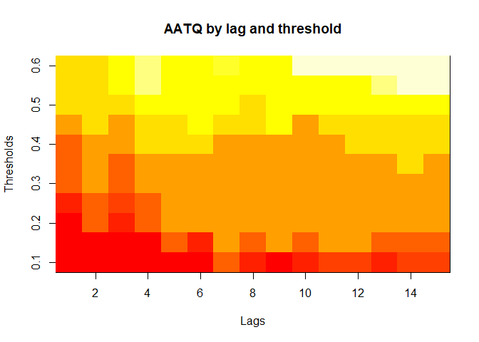
plot(alarm_metrics$metrics, "AATQ")  # Average Alert Time Quality

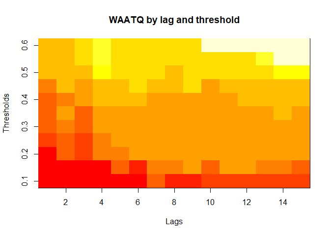
plot(alarm_metrics$metrics, "WAATQ") # Weighted Average Alert Time Quality

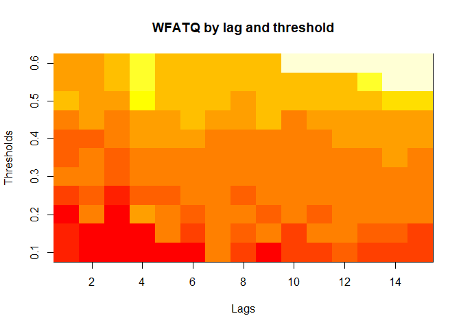
plot(alarm_metrics$metrics, "WFATQ") # Weighted First Alert Time Quality

plot(alarm_metrics$metrics, "ADD")   # Accumulated Delay Days



# Summarize alarm metrics
summary(alarm_metrics$results)
#> Alarm Metrics Summary
#> =====================
#> 
#> FAR :
#>   Mean: 0.5603 
#>   Variance: 0.0191 
#>   Optimal lag: 9 
#>   Optimal threshold: 0.1 
#>   Minimum value: 0.2111 
#> 
#> ADD :
#>   Mean: 25.831 
#>   Variance: 75.0129 
#>   Optimal lag: 1 
#>   Optimal threshold: 0.1 
#>   Minimum value: 6.1111 
#> 
#> AATQ :
#>   Mean: 0.542 
#>   Variance: 0.028 
#>   Optimal lag: 2 
#>   Optimal threshold: 0.1 
#>   Minimum value: 0.1861 
#> 
#> FATQ :
#>   Mean: 0.5451 
#>   Variance: 0.0228 
#>   Optimal lag: 9 
#>   Optimal threshold: 0.1 
#>   Minimum value: 0.1964 
#> 
#> WAATQ :
#>   Mean: 0.5288 
#>   Variance: 0.0313 
#>   Optimal lag: 1 
#>   Optimal threshold: 0.15 
#>   Minimum value: 0.1373 
#> 
#> WFATQ :
#>   Mean: 0.5474 
#>   Variance: 0.0217 
#>   Optimal lag: 4 
#>   Optimal threshold: 0.1 
#>   Minimum value: 0.2516 
#> 
#> Reference Dates and Model Selected Alert Dates:
#> =====================
#> 
#>    year ref_date FAR ADD AATQ FATQ WAATQ WFATQ
#> 1     1       53  NA  NA   NA   NA    NA    NA
#> 2     2       64  50  51   51   50    51    53
#> 3     3       43  42  NA   NA   42    NA    NA
#> 4     4       61  54  51   51   54    51    52
#> 5     5       45  45  33   34   45    33    33
#> 6     6       49  40  35   36   40    35    37
#> 7     7       40  31  31   30   31    37    31
#> 8     8       48  NA  35   41   NA    35    41
#> 9     9       61  55  47   50   55    50    55
#> 10   10       79  72  65   65   72    65    67

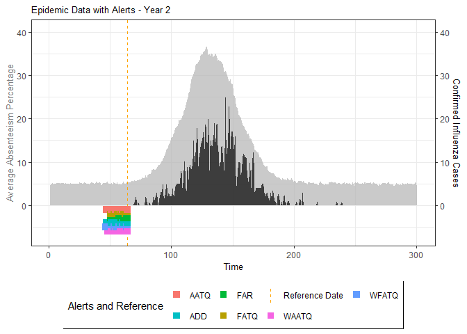
# Generate and display plots for alarm metrics across epidemic years
alarm_plots <- plot(alarm_metrics$plot_data)
for(i in seq_along(alarm_plots)) { 
  print(alarm_plots[[i]]) 
}

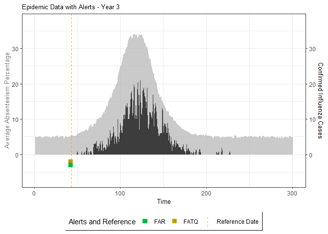
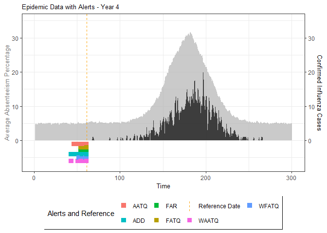
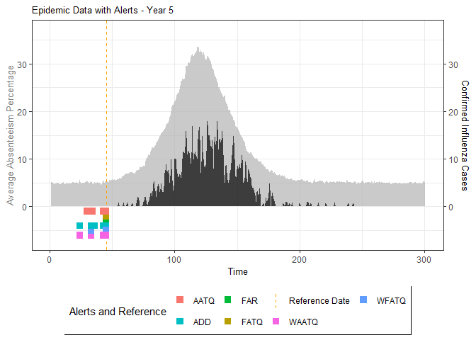
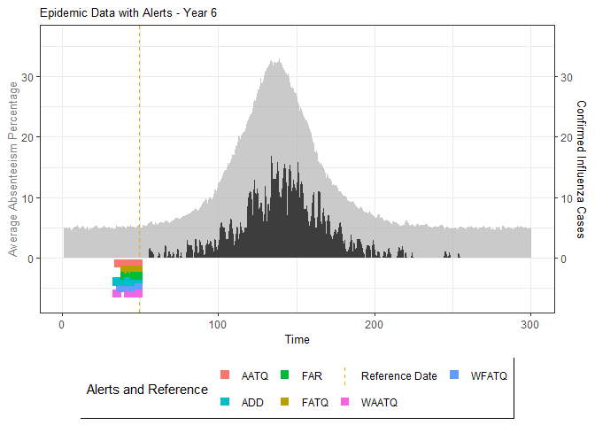
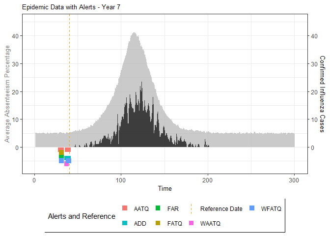
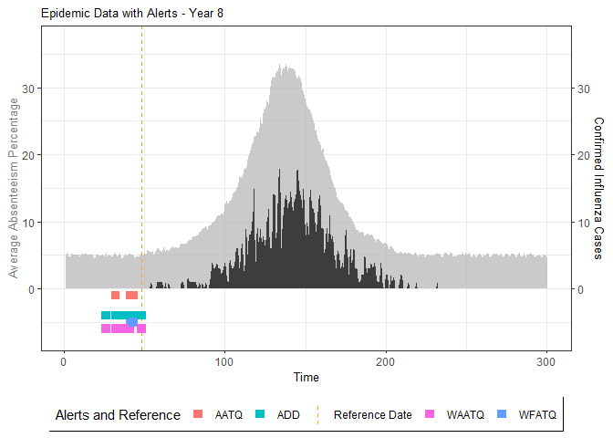
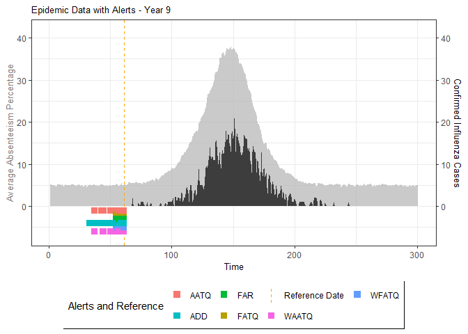
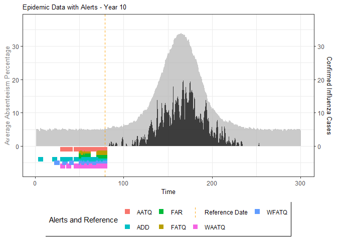
The final output region_metric will be a list of 6 matrices and 6 data frames. The matrices describe the values of metrics for respective lag and thresholds.

An optimal lag and threshold value that minimizes each metric is selected and these optimal parameters are used to generate the 6 data frames associated with the metrics. Simulated information like number of lab confirmed cases, number of students absent, etc, are also included in the output.

r-DESA

DESA: Detecting Epidemics using School Absenteeism <badges go here>

Overview

Why School Absenteeism?

Background

Installation:

Key Functions

Version

License

Status

Source

Homepage

Platforms (75)

DESA: Detecting Epidemics using School Absenteeism <badges go here>

Overview

Why School Absenteeism?

Background

Installation:

Key Functions

Version

License

Status

Source

Homepage

Platforms75 (75)

Platforms (75)