Description

Implementation of the Direct Sampling Spatial Prior.

Description

Draw samples from the direct sampling spatial prior model as described in G. White, D. Sun, P. Speckman (2019) <arXiv:1906.05575>. The basic model assumes a Gaussian likelihood and derives a spatial prior based on thin-plate splines.

README.md

cran.r-project.org

DSSP

The goal of DSSP is to draw samples from the direct sampling spatial prior model (DSSP) described in White et. al. 2019. The basic model assumes a Gaussian likelihood and derives a spatial prior based on thin-plate splines. Functions are included so that the model can be extended to be used for generalised linear mixed models or Bayesian Hierarchical Models.

Installation

You can install the development version from GitHub with:

# install.packages("devtools")
devtools::install_github("gentrywhite/DSSP")

Example

Short example using the Meuse dataset from the {gstat} package.

data("meuse.all", package = "gstat")
sp::coordinates(meuse.all) <- ~ x + y

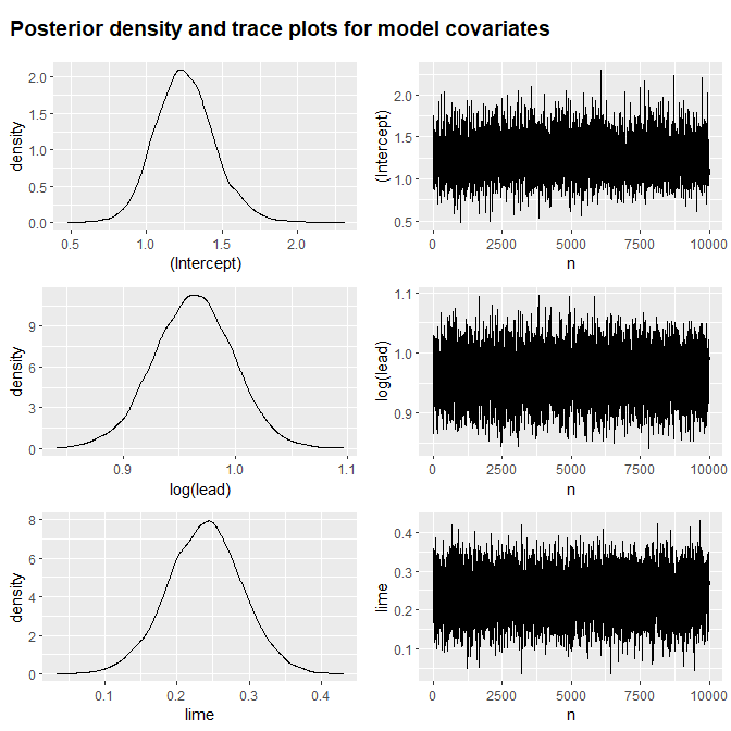
This model does includes two covariates and their posterior densities are summarised in the summary()

library(DSSP)
meuse.fit <- DSSP(
  formula = log(zinc) ~ log(lead) + lime, data = meuse.all, N = 10000,
  pars = c(0.001, 0.001), log_prior = function(x) -2 * log(1 + x)
)
summary(meuse.fit)
#> Formula: log(zinc) ~ log(lead) + lime
#> Number of observations: 164
#> Number of iterations: 10000
#> 
#> Summary of model:
#>       Estimate Est.Error l-95% CI u-95% CI      ESS
#> eta     334.14   1202.47     3.61  1897.49 10000.00
#> delta     0.11      0.01     0.09     0.14 10000.00
#> 
#> Summary of covariates:
#>             Estimate Est.Error  min q0.025 q0.25 q0.50 q0.75 q0.975  max
#> (Intercept)     1.25      0.20 0.48   0.89  1.12  1.25  1.38   1.67 2.30
#> log(lead)       0.96      0.04 0.84   0.89  0.94  0.96  0.99   1.03 1.10
#> lime            0.24      0.05 0.03   0.14  0.20  0.24  0.27   0.34 0.43

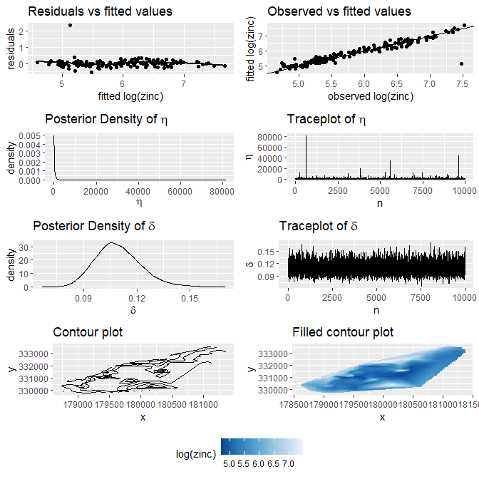
We can inspect several plots for the model using plot().

plot(meuse.fit)
#> `geom_smooth()` using formula 'y ~ x'

Introduction

The Direct Sampling Spatial Prior (DSSP) is based on the thin-plate splines solution to the smoothing problem of minimising the penalised sum of squares

$S_{\eta}(f) = \frac{1}{n}\sum^{n}_{i}W_i(y_i - f(\mathbf{x}_i))^2+\eta J_m(f)$

which can be written as

$\min_{\mathbf{\nu}}\:(\mathbf{y}-\mathbf{\nu})'\mathbf{W}(\mathbf{y}-\mathbf{\nu})+\eta\mathbf{\nu}'\mathbf{M}\mathbf{\nu}.$

The solution for this problem is

$\hat{\mathbf{\nu}}=(\mathbf{W}+\eta\mathbf{M})^{-1}\mathbf{y}.$

If we assume that the observed data are from a Gaussian distribution

$\mathbf{y}\sim N(\mathbf{\nu},\delta\mathbf{W}^{-1})$

and if we specify the prior for $\mathbf{\nu}$

$\left[\mathbf{\nu}\mid\eta,\delta\right]\propto\ \frac{\eta}{\delta}^{-{r}/2}\exp\left(-\frac{\eta}{2\delta}\mathbf{\nu}'\mathbf{M}\mathbf{\nu}\right),$

the resulting posterior of $\nu$ is proportional to

$-\frac{1}{2\delta}\left( (\mathbf{y}-\mathbf{\nu})'\mathbf{W}({\mathbf{y}}-\mathbf{\nu})-\eta\mathbf{\nu}'\mathbf{M}\mathbf{\nu}\right)$

which yields the posterior mean with the same solution as the penalised least squares.

The complete model is specified with a Gaussian likelihood, the improper prior for $\nu$ , an inverse gaussian prior for $\delta$ , and a prior for $\eta$ . With this specification the joint posterior is written

$\pi\left(\mathbf{\nu},\delta_0,\eta|\mathbf{y}\right)\proptof(\mathbf{y}|\mathbf{\nu},\delta)\pi\left(\mathbf{\nu}|\eta,\delta\right)\pi\left(\delta\right)\pi\left(\eta\right).$

Given this it is possible to derive the set of posterior distributions

$\pi\left(\mathbf{\nu}|\delta,\eta,\mathbf{y}\right)\\$

$\pi\left(\delta|\eta,\mathbf{y}\right)\\$

$\pi\left(\eta|\mathbf{y}\right)$

which can be sampled directly in sequence to create a draw from the joint posterior

$\pi\left(\mathbf{\nu},\delta_0,\eta|\mathbf{y}\right).$

This is the heart of what the function DSSP() does[^1].

[^1]: see G. White, D. Sun, P. Speckman (2019) \<arXiv:1906.05575\> for details.

r-DSSP

DSSP

Installation

Example

Introduction

Version

License

Status

Source

Homepage

Platforms (75)

DSSP

Installation

Example

Introduction

Version

License

Status

Source

Homepage

Platforms75 (75)

Platforms (75)