An Extension of the Gap Statistic for Ordinal/Categorical Data.
DiscreteGapStatistic
DiscreteGapStatistic estimates the number of clusters from (multiple choice) categorical response format data given any clustering algorithm extending the well-known gap statistic using a discrete distance based approach.
Installation
You can install the development version of DiscreteGapStatistic from GitHub with:
# install.packages("devtools")
devtools::install_github("ecortesgomez/DiscreteGapStatistic")
Example: Math Anxiety Data
Summarization and Data Exploration
Basic usage of DiscreteGapStatistic is shown using likert’s Math Anxiety data.
library(DiscreteGapStatistic)
library(dplyr)
#>
#> Attaching package: 'dplyr'
#> The following objects are masked from 'package:stats':
#>
#>     filter, lag
#> The following objects are masked from 'package:base':
#>
#>     intersect, setdiff, setequal, union
library(ggplot2)
Libraries are uploaded. Questions are lightly reformatted and the categories are shortened.
## mass dataset is loaded automatically with DiscreteGapStatistic

data(mass)

massSh <- mass[, -1]

sID <- substring(mass$Gender, 1, 1) ## Removing Gender variable
sID[sID == 'F'] <- paste0(sID[sID == 'F'], 1:sum(sID == 'F'))
sID[sID == 'M'] <- paste0(sID[sID == 'M'], 1:sum(sID == 'M'))
rownames(massSh) <- sID

Cats <- setNames(c('SD', 'D', 'N', 'A', 'SA'),
   c('Strongly Disagree', 'Disagree', 'Neutral', 'Agree', 'Strongly Agree') )

massSh <- data.frame(apply(massSh, 2,
   function(x) Cats[as.character(x)] %>%
   factor(levels = Cats)),
   check.names=FALSE, row.names = sID)
colnames(massSh) <- c('Q1: Math Interesting', 'Q2: Uptight Math Test',
   'Q3: Use Math In Future', 'Q4: Mind Goes Blank', 'Q5: Math Relates to Life',
   'Q6: Ability Solve Math Probls', 'Q7: Sinking Feeling', 'Q8: Math Challenging',
   'Q9: Math Makes Me Nervous', 'Q10: Take More Math Classes',
   'Q11: Math Makes Me Uneasy','Q12: Math Favorite Subj.',
   'Q13: Enjoy Learning Math', 'Q14: Math Makes Feel Confused')
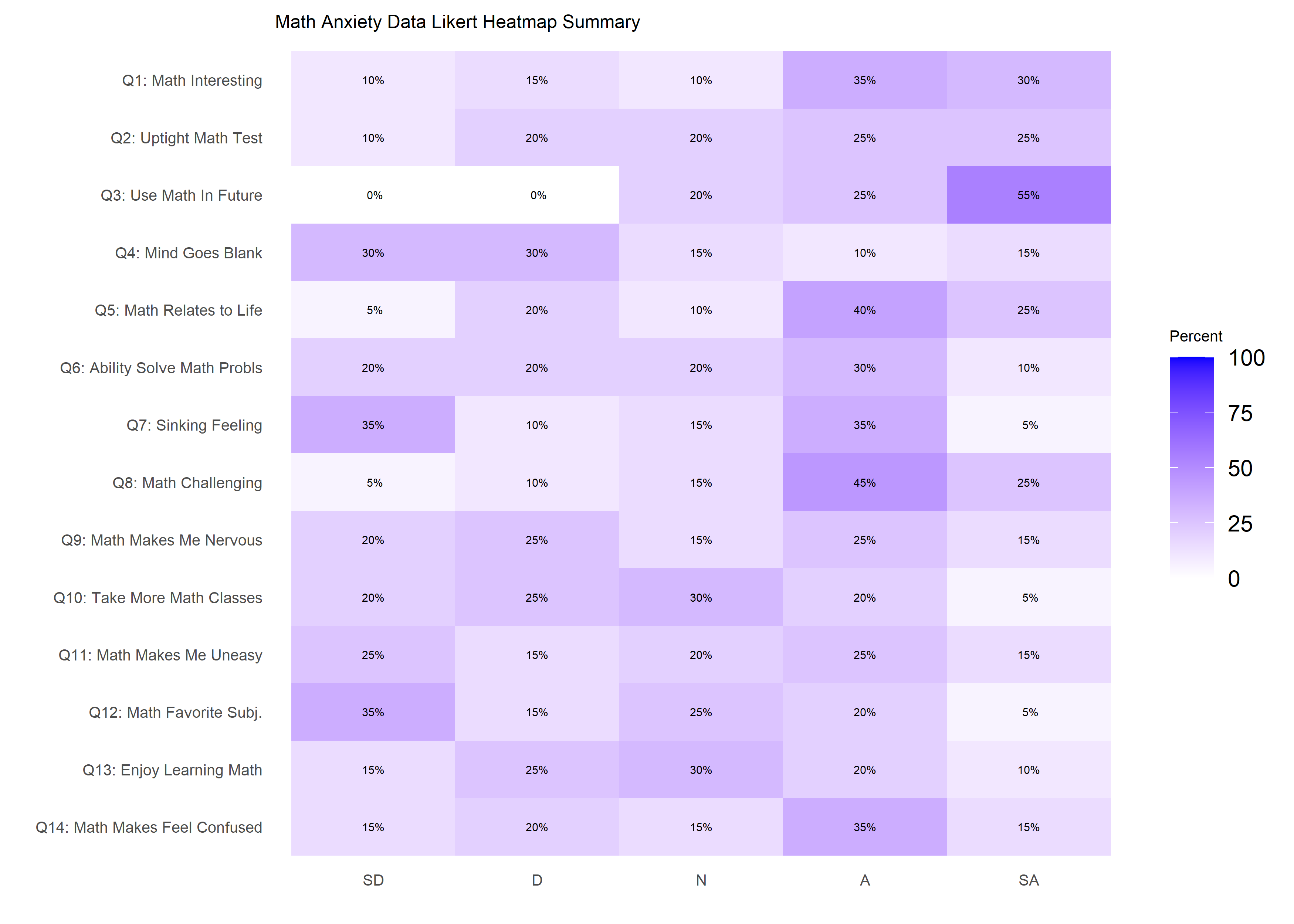
Likert Heatmap
The dataset is visualized using a heatmap similar to the one produced by likert::likert.heatmap.plot.
likert.heat.plot2(massSh,
                  allLevels = Cats,
                  text.size = 1.5)+
   labs(title = 'Math Anxiety Data Likert Heatmap Summary')+
   theme(axis.text = element_text(size = 6),
         title = element_text(size = 6))
Distance Matrices
Five categorical distance functions are introduced to quantify dissimilarities/discrepancies between two categorical vectors (see function distancematrix). The following table describes the available distances and the names used within the package.
#>
#> Attaching package: 'kableExtra'
#> The following object is masked from 'package:dplyr':
#>
#>     group_rows
| Distance | Name |
|---|---|
| Hamming | hamming |
| chi-square | chisquare |
| Cramer’s V | cramerV |
| Hellinger | hellinger |
| Bhattacharyya | bhattacharyya |
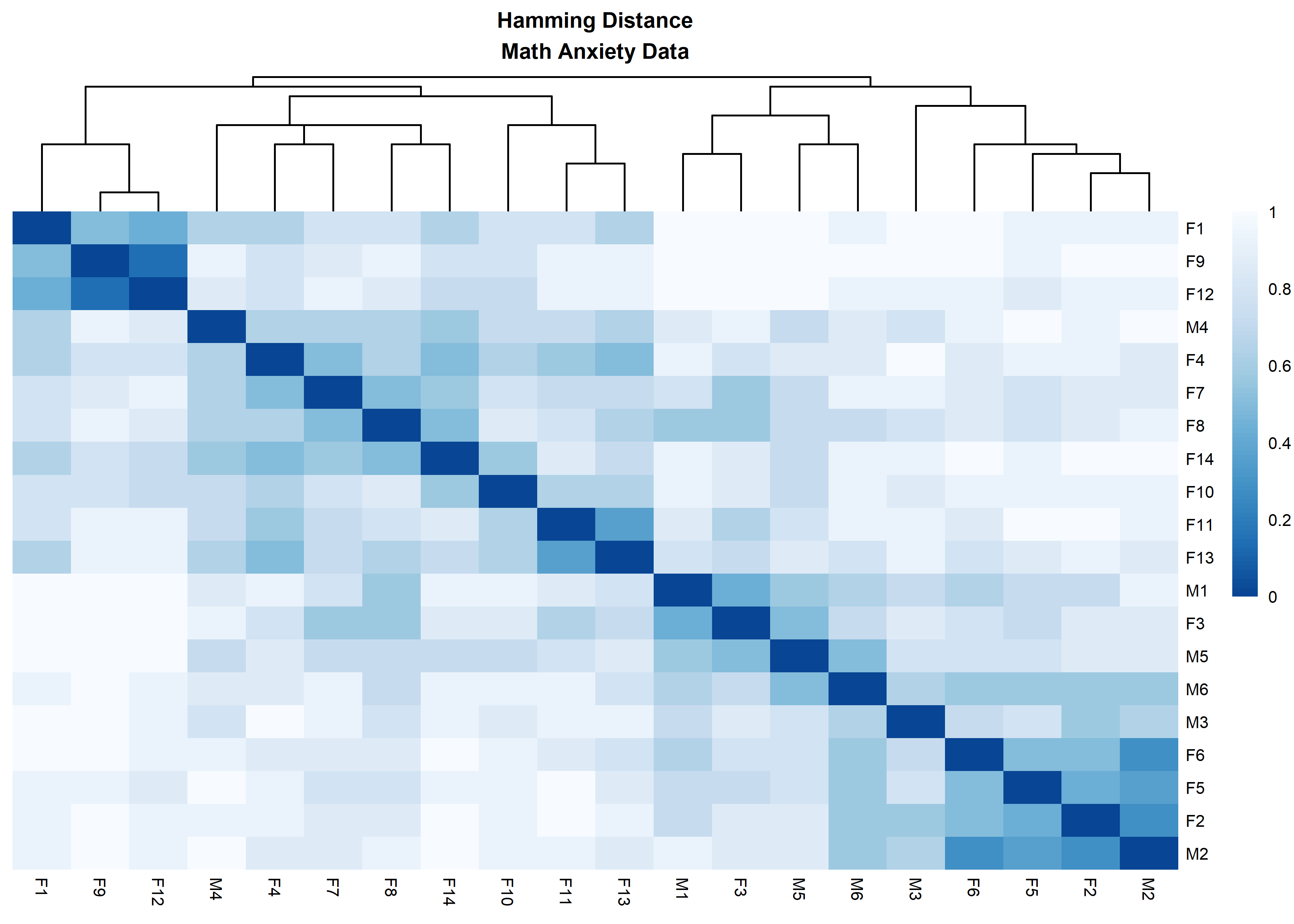
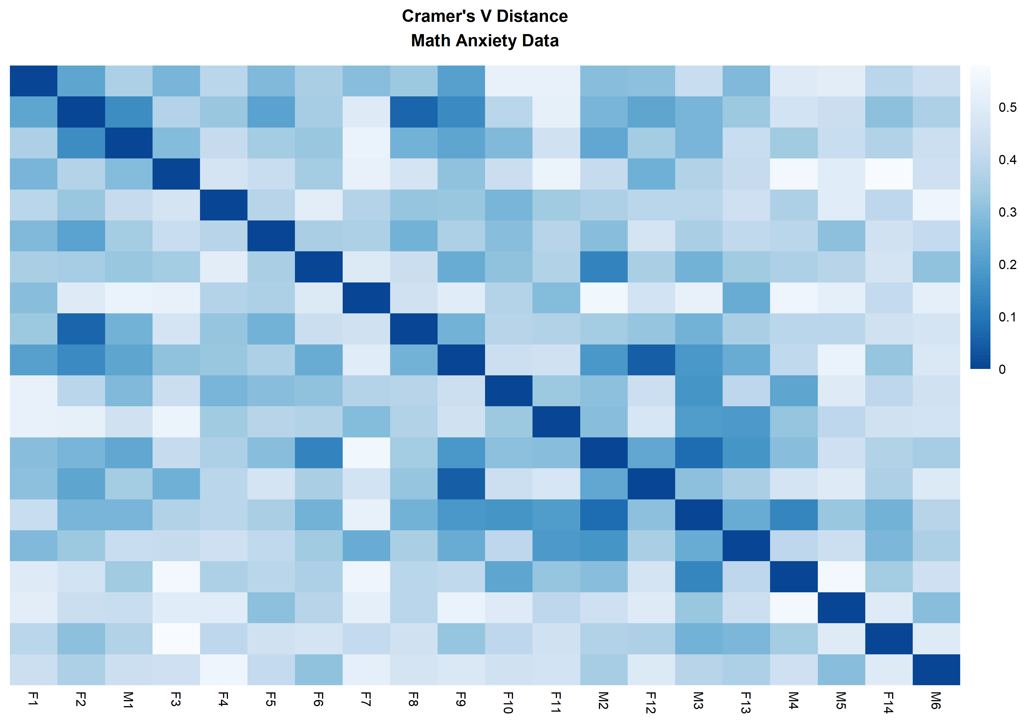
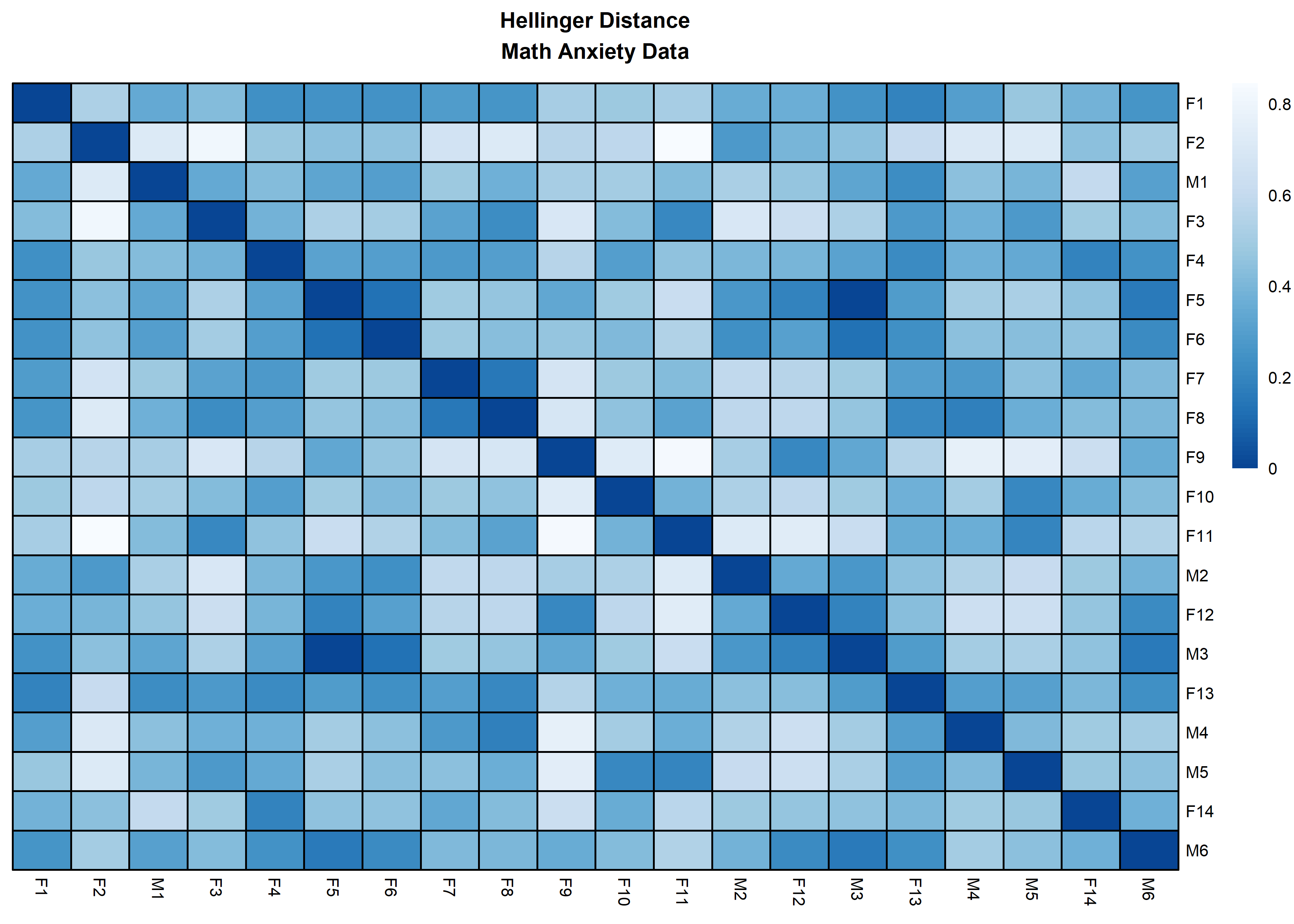
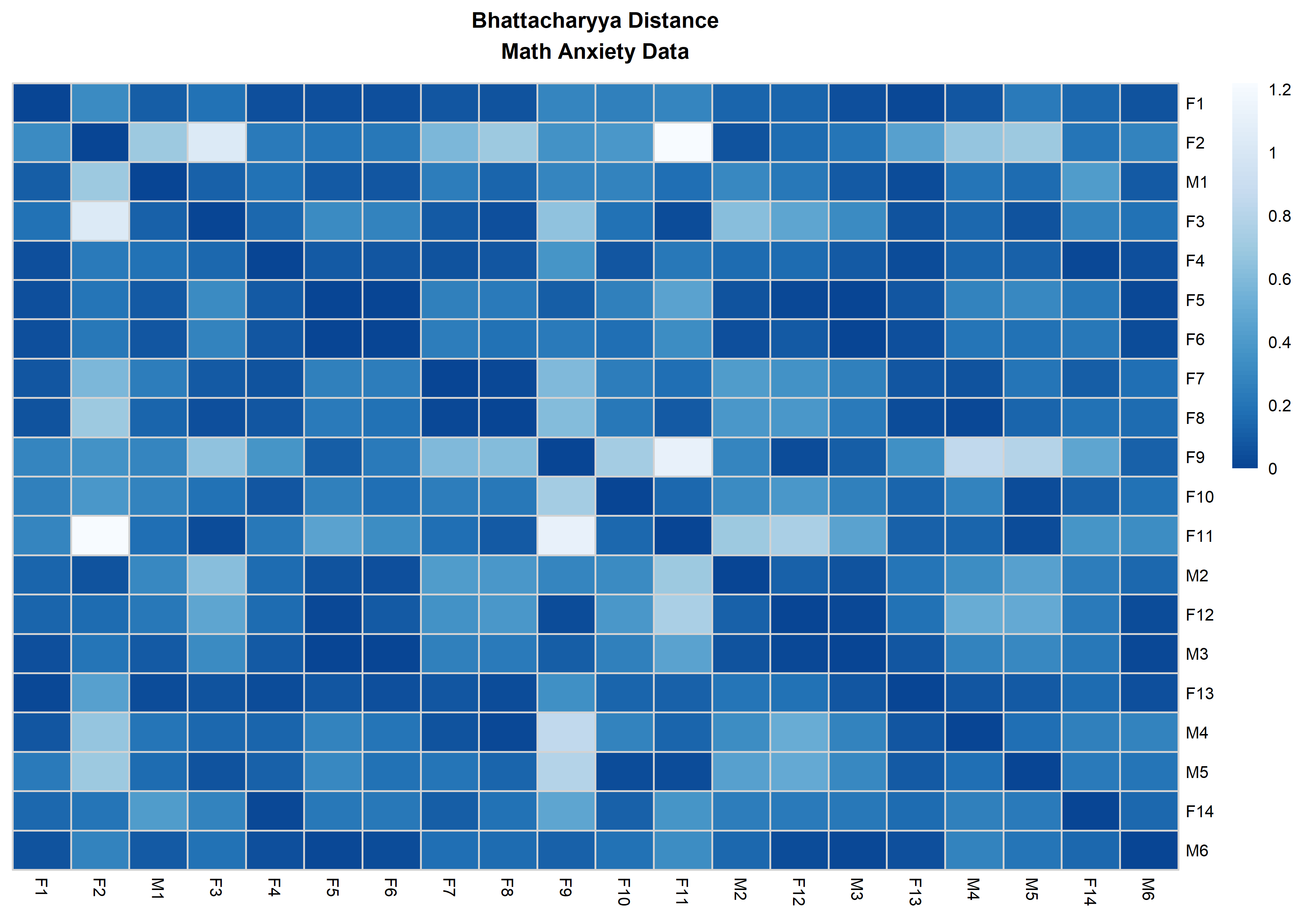
The resulting distance matrix from a rectangular dataset can easily be displayed and organized using heatmaps. The following plots visualize the massData using the defined distances with the function distanceHeat. This function only requires the dataset object and the name of the distance. It can also take advantage of the options and functionalities available in the pheatmap function (see the code below) from the pheatmap R package [@kolde2019]. For instance, by default, the columns are clustered using clustering_method = 'complete' but this parameter can be specified according to pheatmap’s options. Different aesthetic options are exemplified in the plots below using the introduced distances.
distanceHeat(x = massSh,
             distName = 'hamming',
             main = 'Hamming Distance\nMath Anxiety Data',
             fontsize = 6.5)

distanceHeat(x = massSh,
             distName = 'cramerV',
             main = "Cramer's V Distance\nMath Anxiety Data",
             fontsize = 6.5,
             show_rownames = FALSE,
             cluster_rows = FALSE,
             cluster_cols=FALSE)
distanceHeat(x = massSh,
             distName = 'hellinger',
             main = 'Hellinger Distance\nMath Anxiety Data',
             fontsize = 6.5,
             show_rownames = TRUE,
             border_color = 'black',
             cluster_rows = FALSE,
             cluster_cols=FALSE)

distanceHeat(x = massSh,
             distName = 'bhattacharyya',
             main = 'Bhattacharyya Distance\nMath Anxiety Data',
             fontsize = 6.5,
             show_rownames = TRUE,
             border_color = 'lightgrey',
             cluster_rows = FALSE,
             cluster_cols=FALSE)
clusGapDiscr: The Gap Statistic for discrete data
The Gap Statistic (GS) in its original formulation by Tibshirani et. al aims to determine an optimal number of clusters given a rectangular dataset with continuous columns and a pre-specified clustering method given $k$ number of clusters (i.e. $k$-means clustering or partitioning around medoids (pam)). This is done by comparing the within-cluster dispersion of the data to a randomly generated reference null distribution of the data obtaining estimations via bootstrapping. The idea is to quantify whether the clustering structure observed in the data is considerably different compared to what would be expected by random chance. clusGap is a widely used implementation of the GS from the cluster package [@maechler2023cluster] with the following basic arguments:
clusGap(x,
        FUNcluster,
        K.max,
        B = 100,
        verbose = interactive(),
        ...)
x: argument can bedata.frameormatrixobject where rows represent observations and columns correspond to data features or variables. This matrix is expected to be contain exclusively numerical input.FUNcluster: clustering function accepting on its first argument a rectangular data object (likex) and a second one specifying a desiredknumber of clusters.K.max: maximum number of clusters to consider.B: integer indicating the number of times to perform the Montecarlo repetitions.
The discrete GS (dGS) proposed applies and adapts the principle behind the original formulation, but for categorical data using a distance-based approach. The GS assumes that the distance between observations can be correctly described with the Euclidean distance, since it assumes the data is continuous. In the case of categorical data, this distance assumption is not appropriate and a different class of distances needs to be defined. clusGapDiscr is the main function that performs and implements dGS. Parameters x, K.max and B found in clusGapDiscr have the same meaning and usage to the ones found in clusGap. clusterFUN expects the name of a well-known clustering algorithm implementation available in R amenable to the proposed methodology. The input options available for this parameter are the following:
| clusterFUN | Package |
|---|---|
| pam | cluster |
| fanny | cluster |
| diana | cluster |
| agnes-{average, single, complete, ward, weighted} | cluster |
| hclust-{average, single, complete, ward.D, ward.D2, mcquitty, median, centroid} | stats |
| kmodes-{1, 2, …, } | klaR |
The first four options are straight-forward since originally these functions can output a clustering partition providing a distance matrix and a given number of clusters. The following two implementations use a flexible hierarchical clustering strategy. The number of desired clusters can be obtained appropriately by cutting the resulting hierarchical tree. This parameter requires the name of the implementation and a dash (-) followed by the exact name of the clustering strategy described in the package corresponding R package. Lastly, a k-modes implementation is included using code found on klaR with options fast=TRUE, weighted = FALSE. The expected string after the dash is a non-negative integer specifying the maximum number of iterations to carry out within the algorithm (iter.max option; inputting kmodes alone runs iter.max = 10 by default).
Additionally, the function requires a categorical distance from the list mentioned above. Another feature of the dGS is the reference null distribution used, which can be a discrete uniform distribution of the unique column-wise categories found in the data; this setting is defined as the Data Support (DS). In other settings, the categories to be used must be user-specified via a character vector or list. This setting will be referred as the Known Support (KS).
clusGapDiscr(x,
             clusterFUN,
             K.max,
             B = nrow(x),
             distName,
             value.range = 'DS',
             verbose = interactive(),
             useLog = TRUE ...)
distName: name of discrete distance. The available options are'hamming','chisquare','cramersV','bhattacharyya'and'hellinger'.value.range: specifies the values of the reference null distribution. Possible values:'DS'or a character vector with unique values.'DS'option extracts the unique values found inx.useLog: Binary truth variable specifying whether to evaluate the Gap Statistic with or without $log$ function.
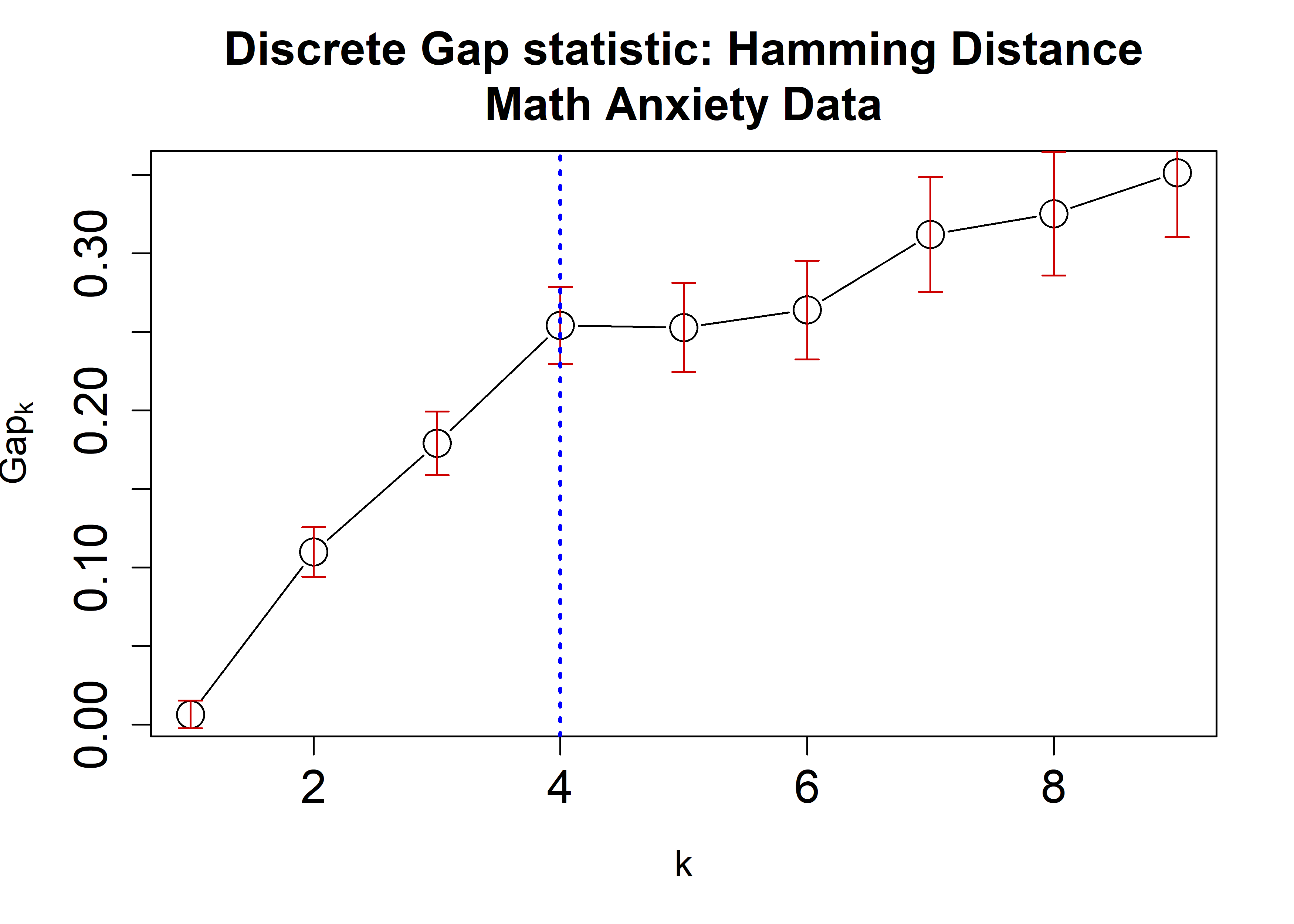
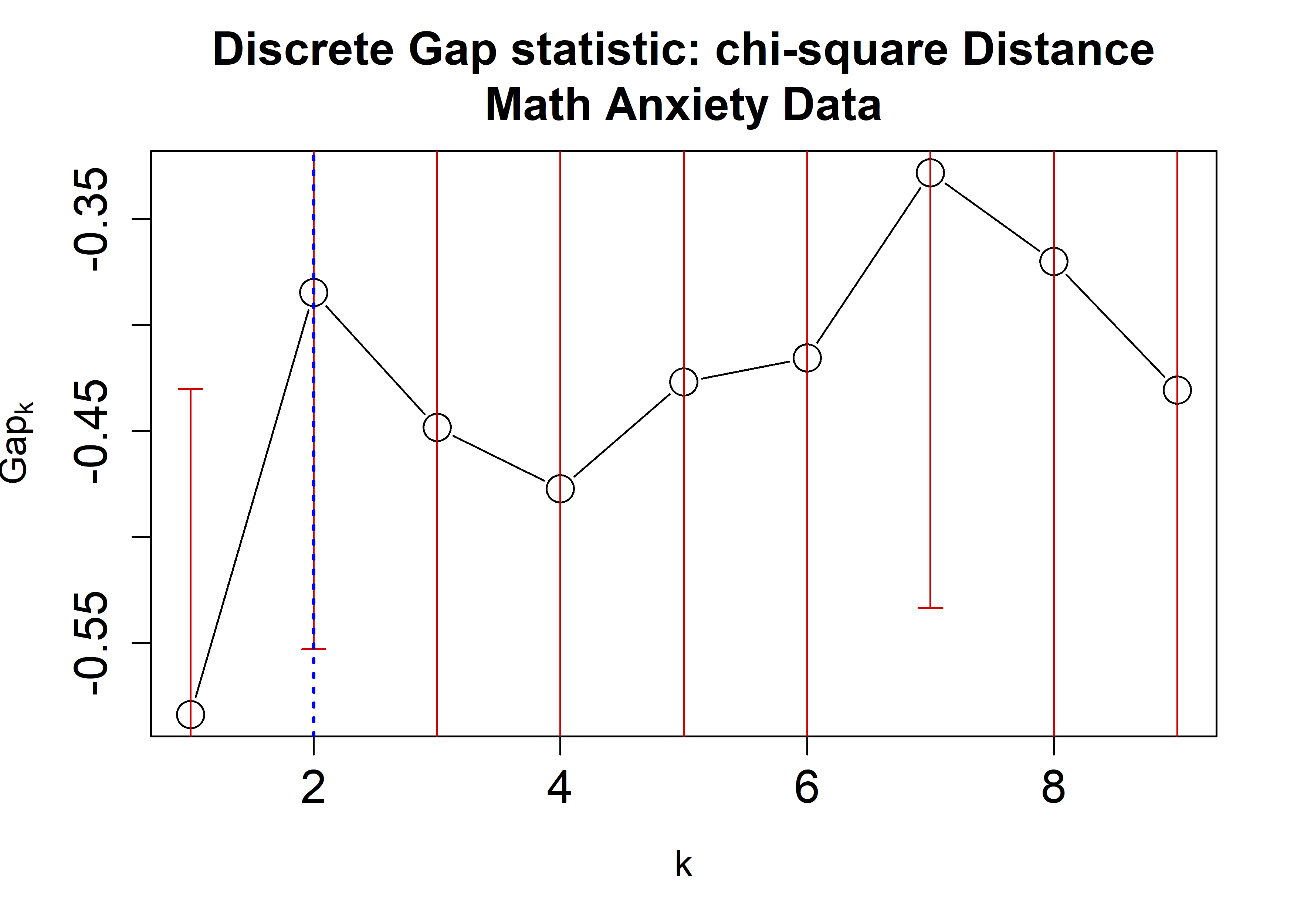
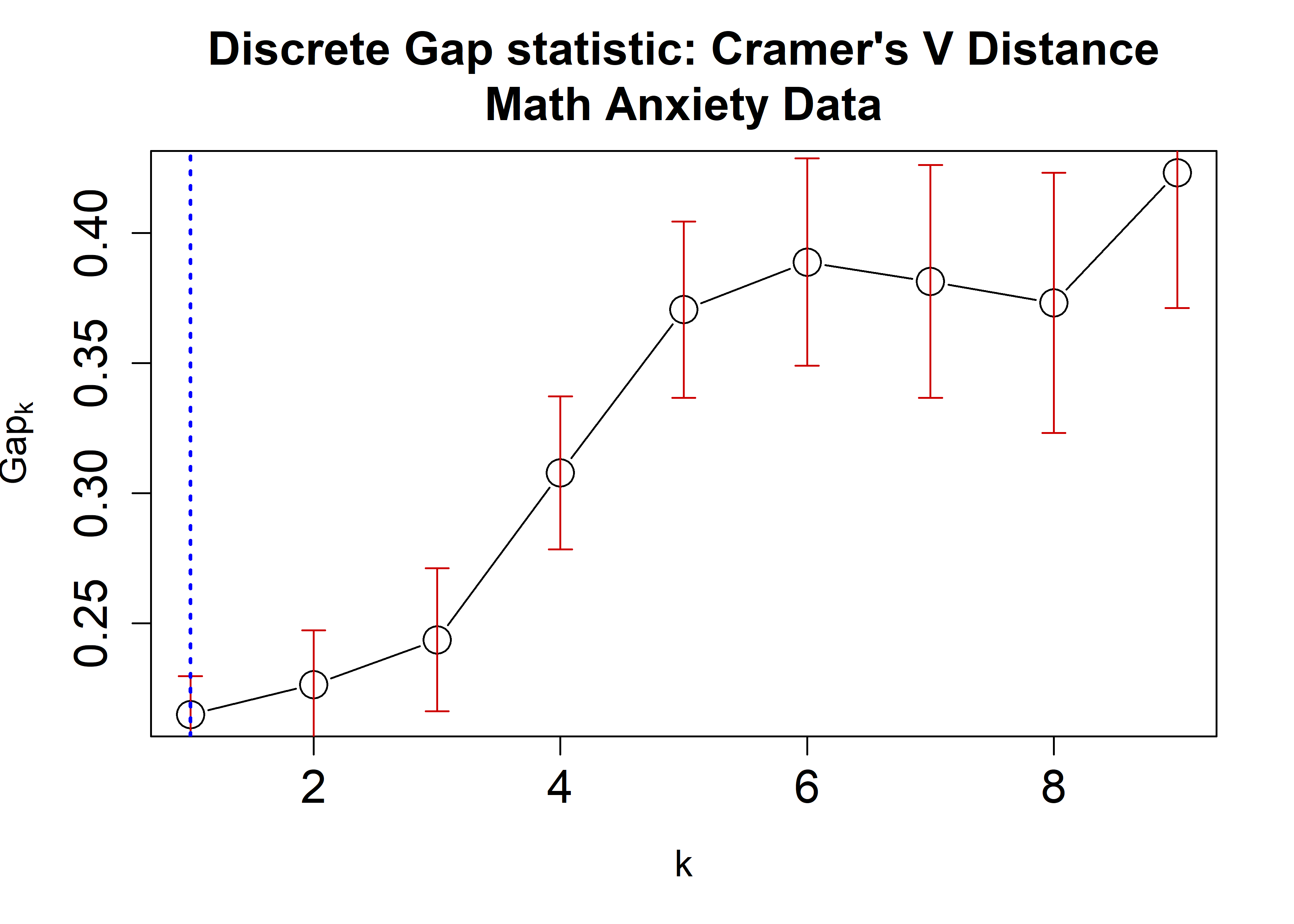
Similar to clusGap, clusGapDiscr returns a matrix object with K.max rows corresponding to the user-specified number of clusters with an estimate of the GS and its corresponding standard error. This information would then determine the number of clusters according to the cluster-selection criterion. The one used in DiscreteGapStatistic is the 1-SE criterion implemented by the function findK, which accepts clusGap objects. The following example applies the dGS on the Math Anxiety data using the Hamming, $\chi^2$, and Cramer’s V distances applying the cluster::pam algorithm. A plot is then generated displaying the dGS against the number of clusters. Each estimate is accompanied by corresponding standard-error bars and a blue dashed line indicating the chosen number of clusters.
Basics
The math anxiety data is further explored under different categorical distances using the cluster::pam algorithm. The number of bootstraps B is increased to 100 since the sample size for this dataset is not too large. The maximum number of clusters to consider is 9.
## Recall Cats:
# Cats <- setNames(object = c('SD', 'D', 'N', 'A', 'SA'),
#                  nm = c('Strongly Disagree', 'Disagree',
#                         'Neutral',
#                         'Agree', 'Strongly Agree') )

HammRun <- clusGapDiscr(x = massSh,
                        clusterFUN = 'pam',
                        B = 100,
                        K.max = 9,
                        value.range = 'DS',
                        distName = 'hamming')
#> Found levels: A, D, N, SA, SD
chisqRun <- clusGapDiscr(x = massSh,
                        clusterFUN = 'pam',
                        B = 100,
                        K.max = 9,
                        value.range = Cats,
                        distName = 'chisquare')
#> Found levels: A, D, N, SA, SD
crVRun <- clusGapDiscr(x = massSh,
                        clusterFUN = 'pam',
                        B = 100,
                        K.max = 9,
                        value.range = 'DS',
                        distName = 'cramerV')
#> Found levels: A, D, N, SA, SD
plot(HammRun,
     main = "Discrete Gap statistic: Hamming Distance\nMath Anxiety Data",
     cex = 2,
     cex.lab=1.2,
     cex.axis=1.5,
     cex.main=1.5)
abline(v = findK(HammRun), lty=3, lwd=2, col="Blue")

plot(chisqRun,
     main = "Discrete Gap statistic: chi-square Distance\nMath Anxiety Data",
     cex = 2,
     cex.lab=1.2,
     cex.axis=1.5,
     cex.main=1.5)
abline(v = findK(chisqRun), lty=3, lwd=2, col="Blue")

plot(crVRun,
     main = "Discrete Gap statistic: Cramer's V Distance\nMath Anxiety Data",
     cex = 2,
     cex.lab=1.2,
     cex.axis=1.5,
     cex.main=1.5)
abline(v = findK(crVRun), lty=3, lwd=2, col="Blue")
Notice that since all possible categorical values are available in the data, using the option value.range = Cats would yield exact same results.
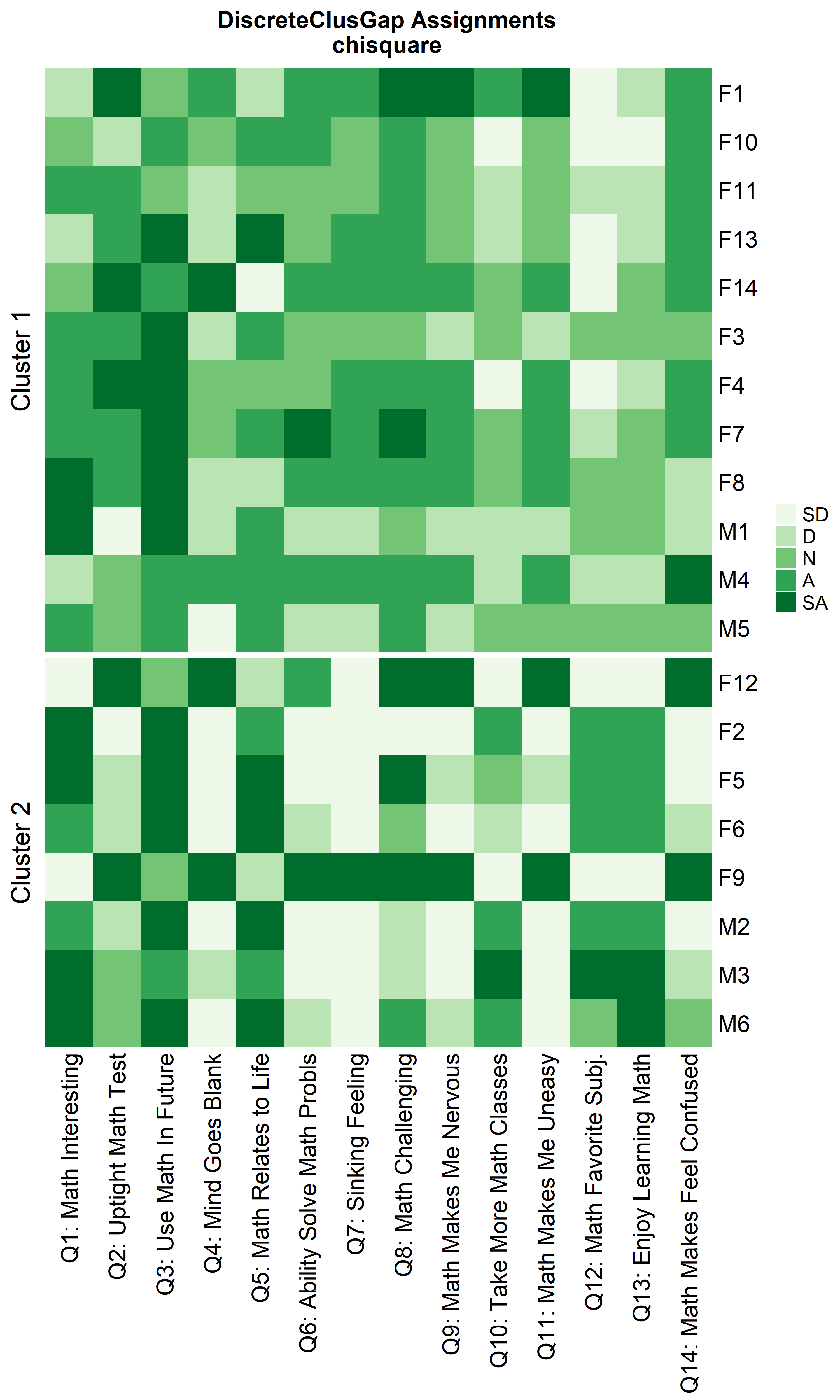
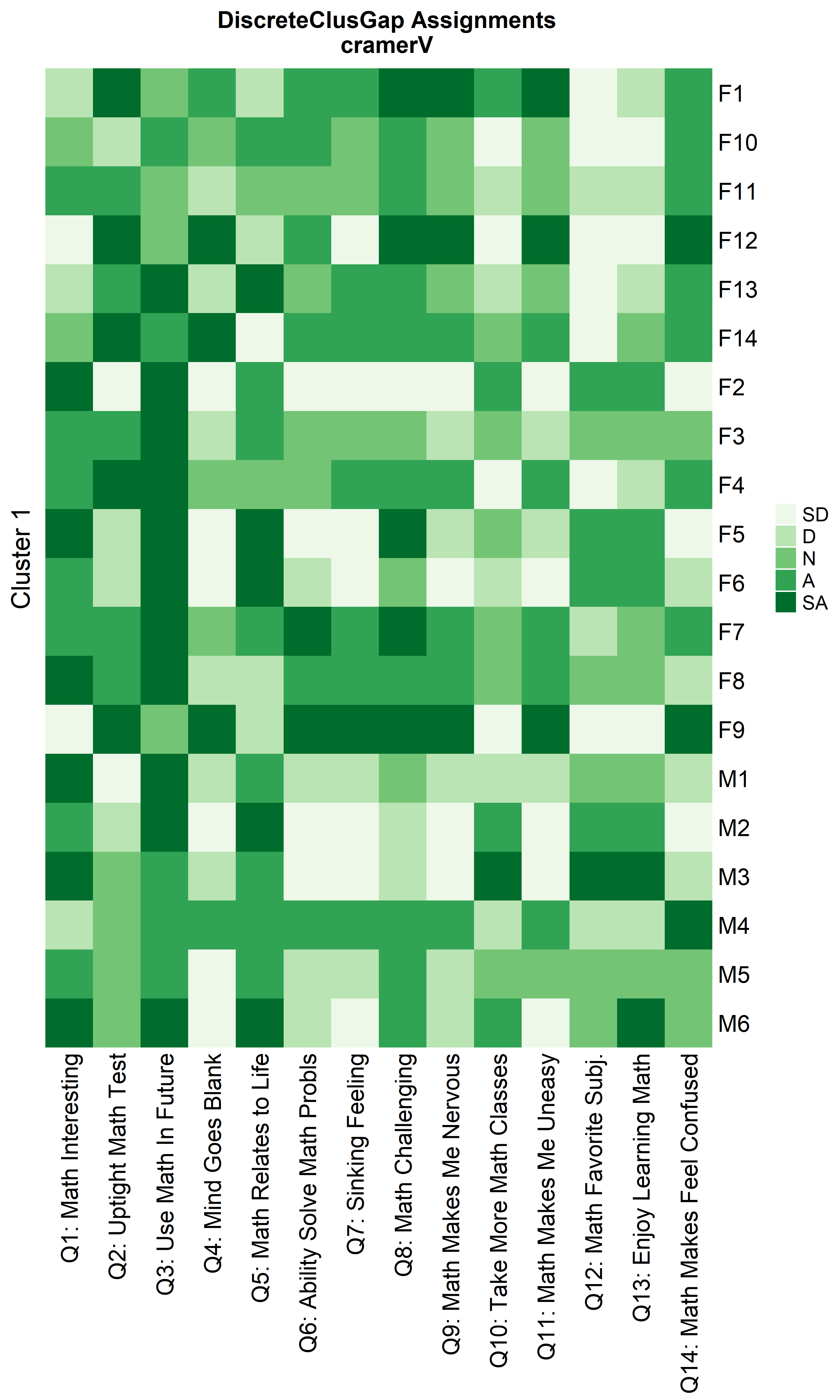
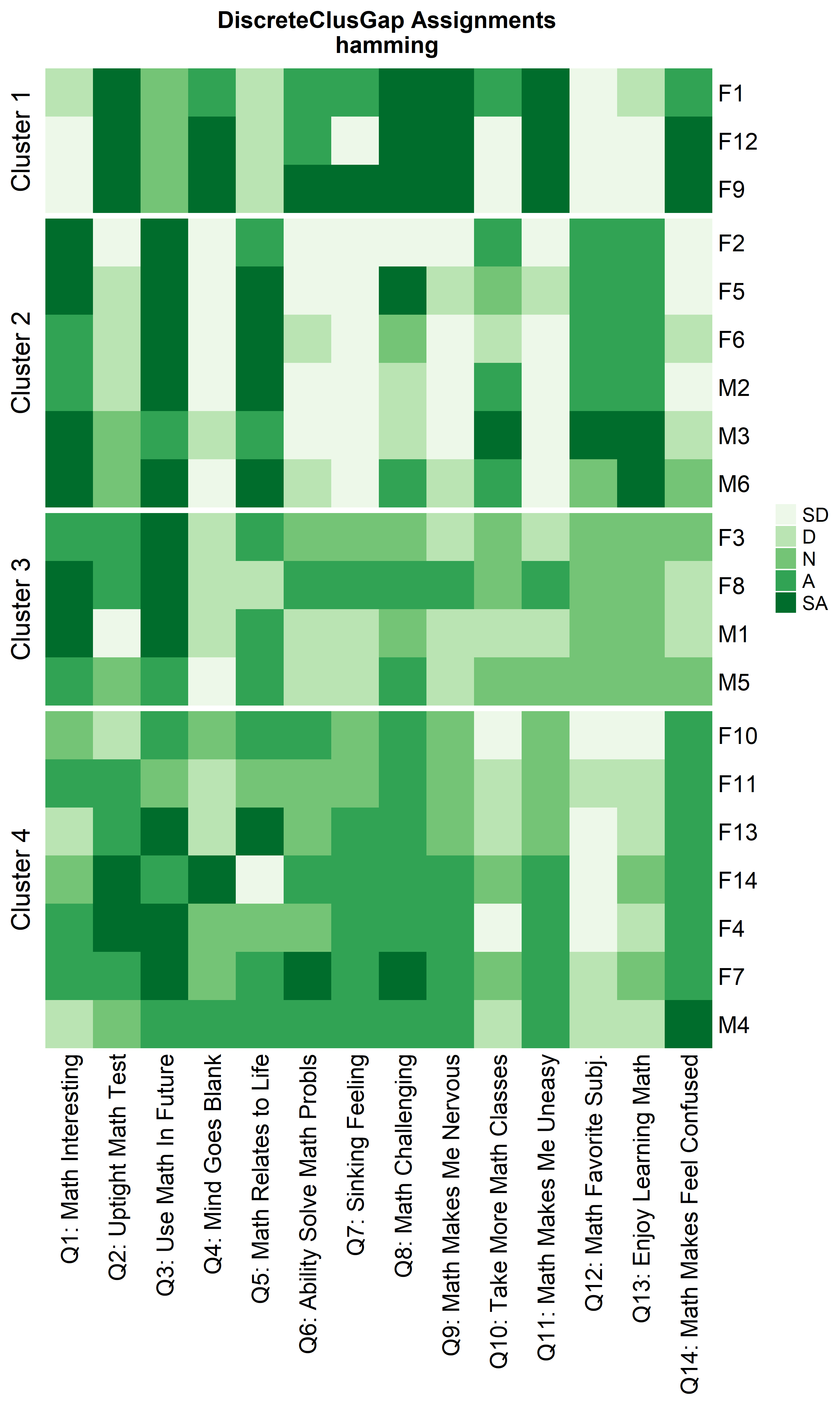
Heatmaps can be created to visualize the commonalities within each cluster and the differences between them.
ResHeatmap(x = massSh,
           distName = 'hamming',
           clusterFUN = 'pam',
           catVals = Cats,
           nCl = findK(HammRun),
           out = 'heatmap',
           prefObs = NULL, height = 6)
#> Warning: The input is a data frame-like object, convert it to a matrix.
#> Warning: Note: not all columns in the data frame are numeric. The data frame
#> will be converted into a character matrix.
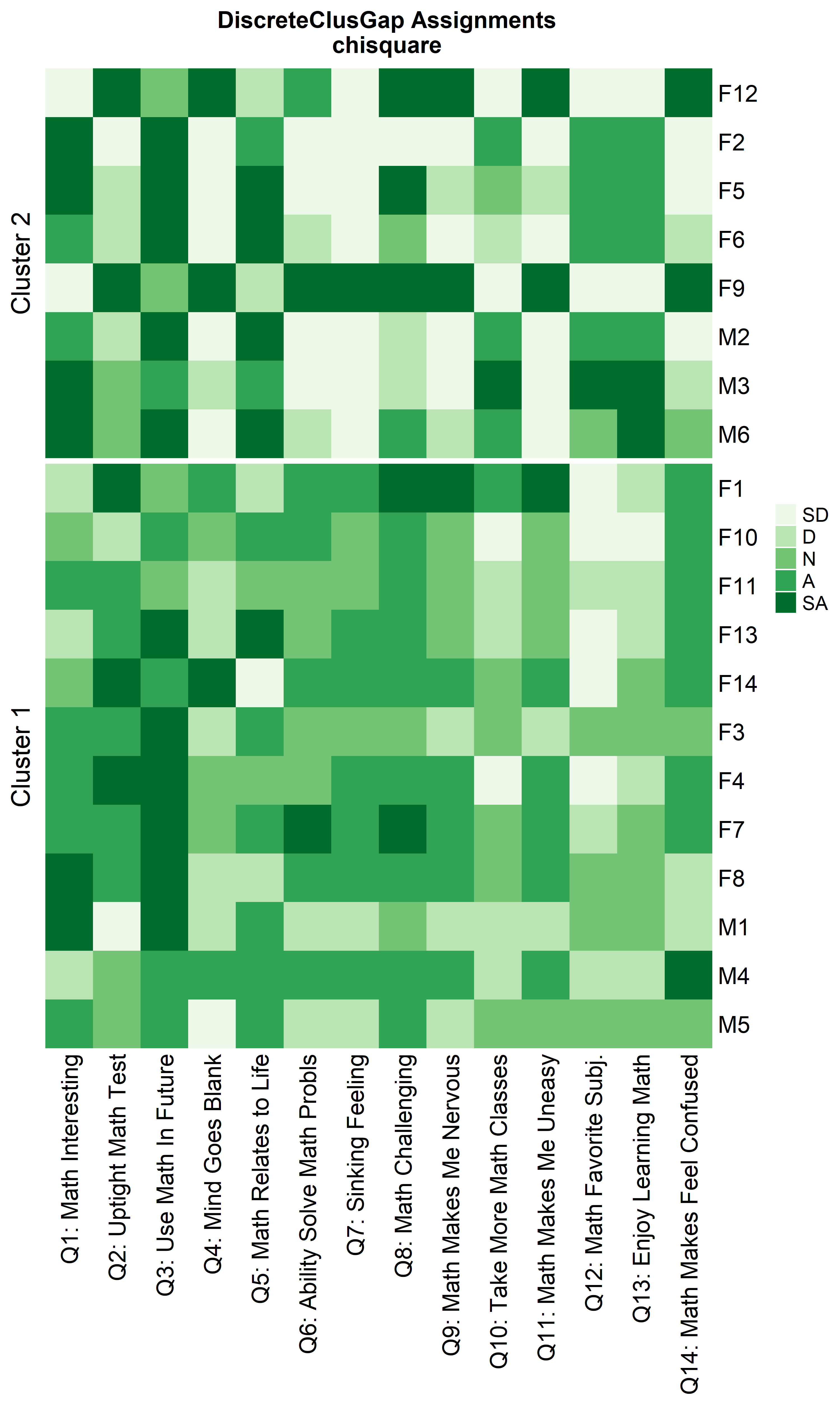
ResHeatmap(x = massSh,
           clusterFUN = 'pam',
           distName = 'chisquare',
           catVals = Cats,
           nCl = findK(chisqRun),
           out = 'heatmap',
           prefObs = NULL, height = 6)
#> Warning: The input is a data frame-like object, convert it to a matrix.
#> Warning: Note: not all columns in the data frame are numeric. The data frame
#> will be converted into a character matrix.
ResHeatmap(x = massSh,
           clusterFUN = 'pam',
           distName = 'cramerV',
           catVals = Cats,
           nCl = findK(crVRun),
           out = 'heatmap',
           prefObs = NULL, height = 6)
#> Warning: The input is a data frame-like object, convert it to a matrix.
#> Warning: Note: not all columns in the data frame are numeric. The data frame
#> will be converted into a character matrix.

Re-arranging clusters
Notice that Hamming distance detects subclusters present in Cluster 2 from the $\chi^2$ distance run. To compare the similar clusters side-to-side, the parameter nCl can be used to reorder the clusters relative to the given ordering. This case nCl = 2:1 will alter (invert) the order of the two clusters on the $\chi^2$ based cluster. A third heatmap is displayed relabeling the clusters from the $\chi^2$ run using the clusterNames = 'renumber' argument.
ResHeatmap(x = massSh,
           clusterFUN = 'pam',
           distName = 'hamming',
           catVals = Cats,
           nCl = findK(HammRun),
           out = 'heatmap',
           height = 6)

ResHeatmap(x = massSh,
           clusterFUN = 'pam',
           distName = 'chisquare',
           catVals = Cats,
           nCl = 2:1,
           out = 'heatmap',
           height = 6)

ResHeatmap(x = massSh,
           clusterFUN = 'pam',
           distName = 'chisquare',
           catVals = Cats,
           nCl = 2:1,
           clusterNames = 'renumber',
           out = 'heatmap',
           height = 6)

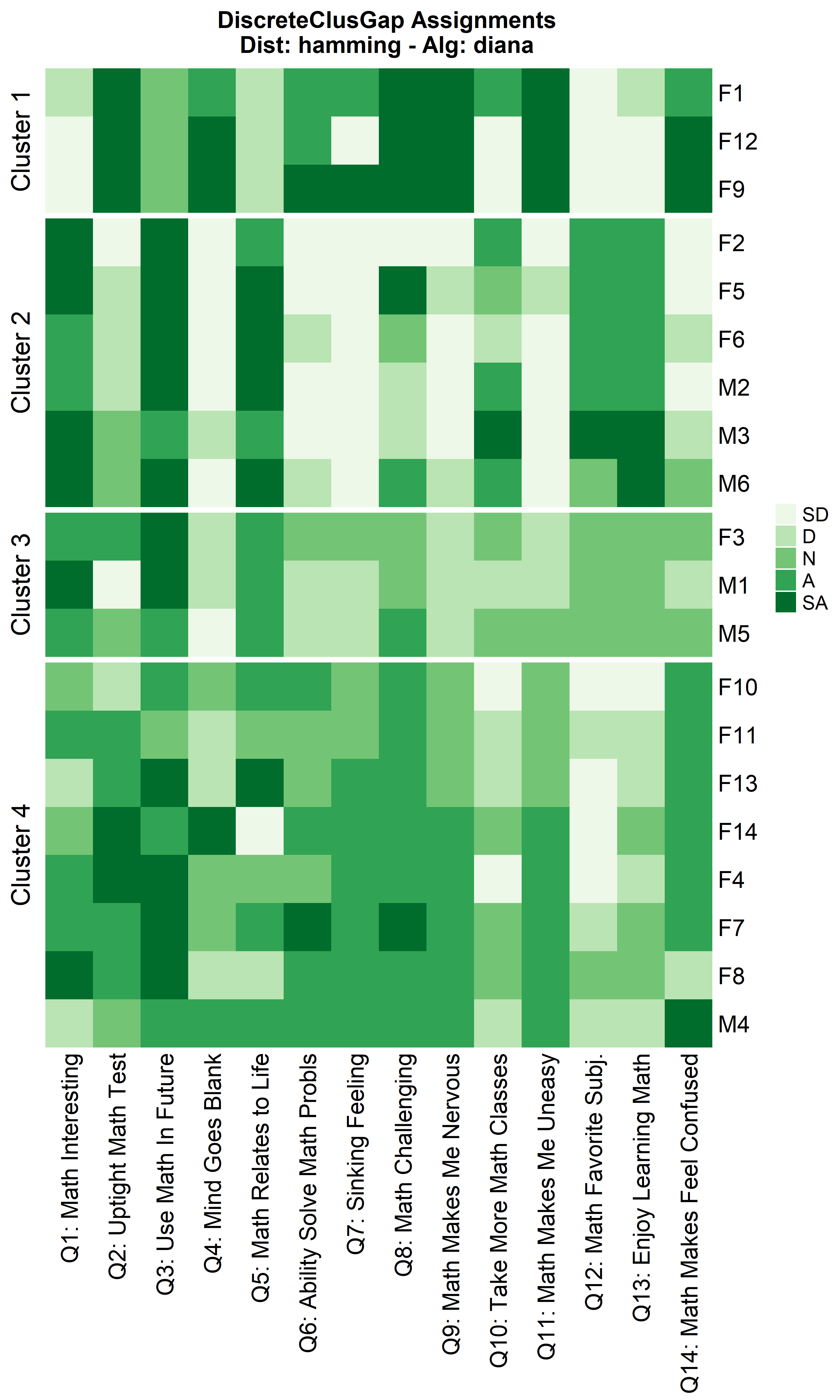
Alternative clustering algorithms
Other compatible clustering algorithms are considered additional to cluster::pam only using the Hamming distance.
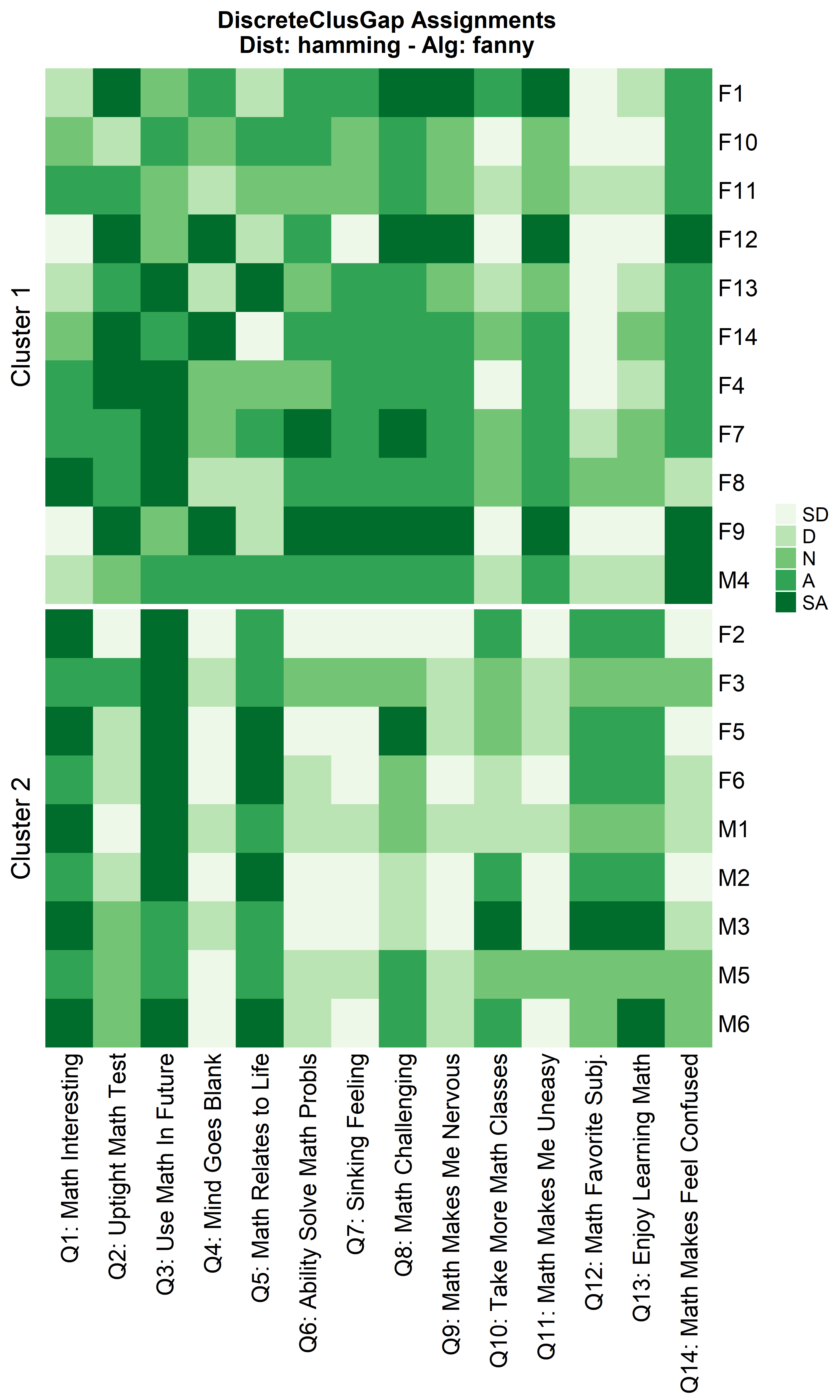
Other cluster algorithms: diana and fanny
hDiaMa <- clusGapDiscr(massSh,
                       clusterFUN = 'diana',
                       K.max = 9,
                       B = 100)
ResHeatmap(x = massSh,
           distName = 'hamming',
           clusterFUN = 'diana',
           catVals = Cats,
           nCl = findK(hDiaMa),
           out = 'heatmap',
           height = 6)

hFanMa <- clusGapDiscr(massSh,
                       clusterFUN = 'fanny',
                       K.max = 9,
                       B = 100)
ResHeatmap(x = massSh,
           clusterFUN = 'fanny',
           distName = 'hamming',
           catVals = Cats,
           nCl = findK(hFanMa),
           out = 'heatmap',
           height = 6)
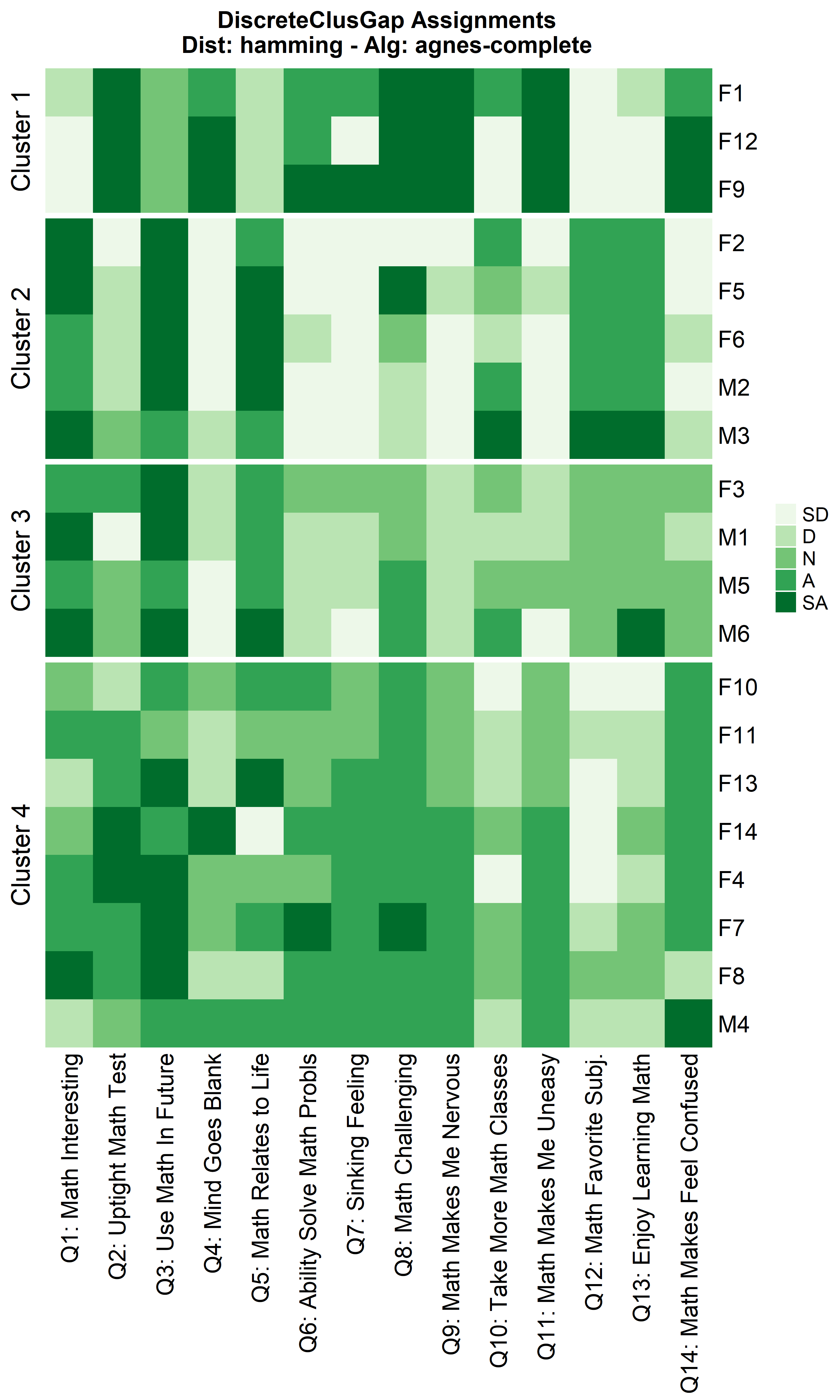
Hierarchical Clustering
hAgnComMa <- clusGapDiscr(massSh,
clusterFUN = 'agnes-complete',
K.max = 9,
B = 100)
ResHeatmap(x = massSh,
distName = 'hamming',
clusterFUN = 'agnes-complete',
catVals = Cats,
nCl = findK(hAgnComMa),
out = 'heatmap',
height = 6)
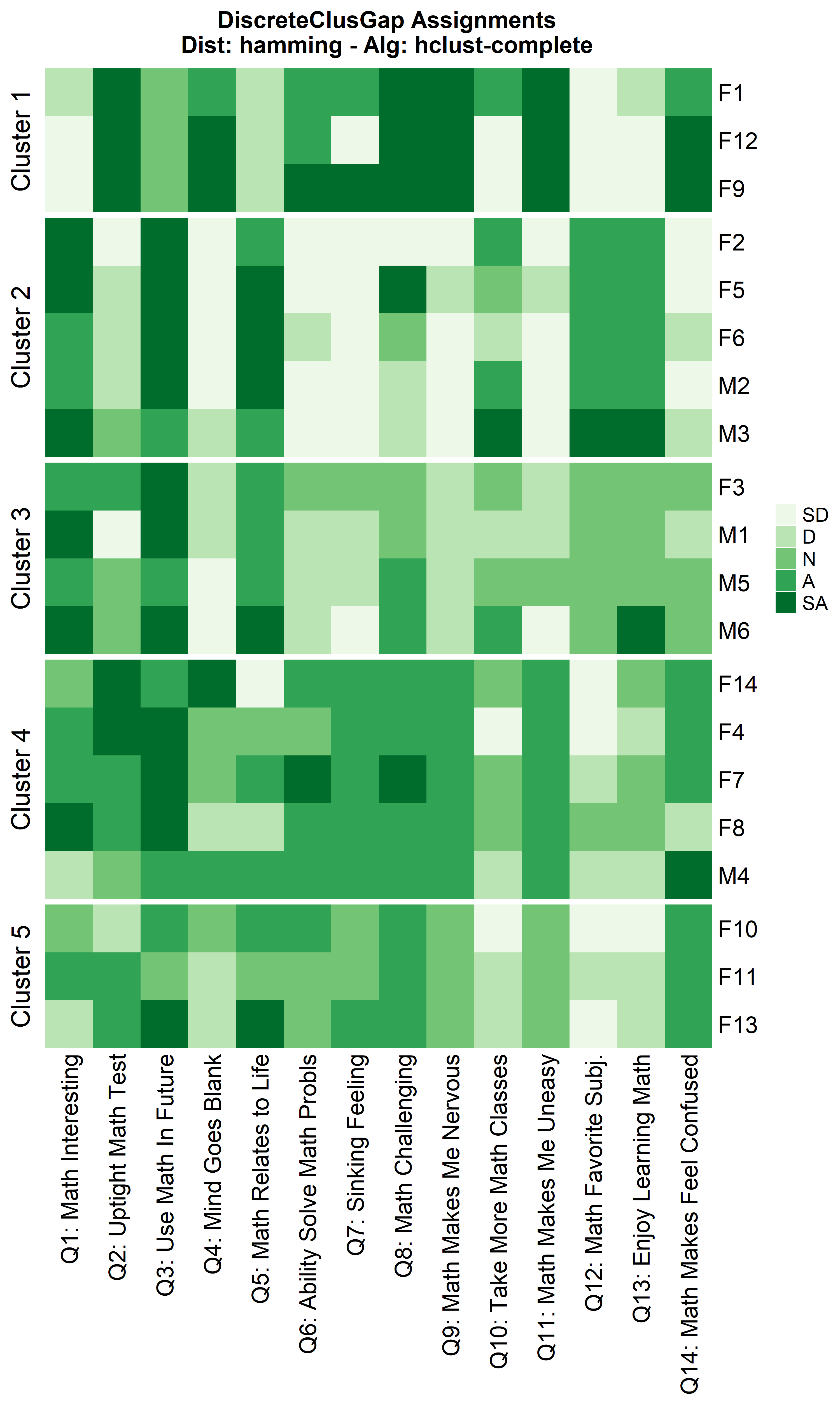
hhclComMa <- clusGapDiscr(massSh,
clusterFUN = 'hclust-complete',
K.max = 9,
B = 100)
ResHeatmap(x = massSh,
distName = 'hamming',
clusterFUN = 'hclust-complete',
catVals = Cats,
nCl = findK(hhclComMa),
out = 'heatmap',
height = 6)
hhclMcqMa <- clusGapDiscr(massSh,
clusterFUN = 'hclust-mcquitty',
K.max = 9,
B = 100)
ResHeatmap(x = massSh,
distName = 'hamming',
clusterFUN = 'hclust-mcquitty',
catVals = Cats,
nCl = findK(hhclMcqMa),
out = 'heatmap',
height = 6)