Bayesian Modal Regression Based on the GUD Family.
Installation
The GUD package provides probability density functions and sampling algorithms for three key distributions from the General Unimodal Distribution (GUD) family: the Flexible Gumbel (FG) distribution, the Double Two-Piece (DTP) Student-t distribution, and the Two-Piece Scale (TPSC) Student-t distribution. Additionally, this package includes a function for Bayesian linear modal regression, leveraging these three distributions for model fitting.
You can install the GUD package:
if (! require(GUD)) {
  install.packages(pkgs = "GUD",
                   repos = "https://cran.rstudio.com/" )
} else {
  require(GUD)
}
#> Loading required package: GUD
Introduction
The general unimodal distribution (GUD) family is essentially a family of two-component mixture distributions. The probability density function (pdf) of a member of GUD family is $$ f\left(y \mid w, \theta, \boldsymbol{\xi}_1, \boldsymbol{\xi}_2\right)=w f_1\left(y \mid \theta, \boldsymbol{\xi}_1\right)+(1-w) f_2\left(y \mid \theta, \boldsymbol{\xi}_2\right), $$ where $w \in [0,1]$ is the weight parameter, $\theta \in (-\infty, +\infty)$ is the mode as a location parameter, $\boldsymbol{\xi}_1$ consists of parameters other than the location parameter in $f_1\left(\cdot \mid \theta, \boldsymbol{\xi}_1\right)$ and $\boldsymbol{\xi}_2$ is defined similarly for $f_2\left(\cdot \mid \theta, \boldsymbol{\xi}_2\right)$. Besides unimodality, all members of the GUD family share three features:
- The pdfs $f_1\left(\cdot \mid \theta, \boldsymbol{\xi}_1\right)$ and $f_2\left(\cdot \mid \theta, \boldsymbol{\xi}_2\right)$ are unimodal at $\theta$.
- The pdfs $f_1\left(\cdot \mid \theta, \boldsymbol{\xi}_1\right)$ and $f_2\left(\cdot \mid \theta, \boldsymbol{\xi}_2\right)$ are left-skewed and right-skewed respectively.
- The mixture pdf $f\left(\cdot \mid w, \theta, \boldsymbol{\xi}_1, \boldsymbol{\xi}_2\right)$ in (1) is continuous in its domain.
More details of the GUD family can be found in Liu, Q., Huang, X., & Bai, R. (2024).
Bayesian Modal Regression Analysis of 2003 United States Crime Data
In this section, we demonstrate how to use the GUD package to analyze 2003 United States Crime Data as in Section 2 of Liu, Q., Huang, X., & Bai, R. (2024).
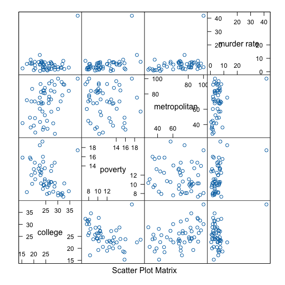
In “The Art and Science of Learning from Data, 5th edition” by Alan Agresti, Christine A. Franklin, and Bernhard Klingenberg, an interesting example about the 2003 United States crime data is presented to demonstrate the influence of outliers in the classic linear regression model. This example is very compelling and partially motivates the construction of the Bayesian modal regression based on the GUD family. This data contains the murder rate, percentage of college education, poverty percentage, and metropolitan rate for the 50 states in the United States and the District of Columbia (D.C.) from 2003. The murder rate is defined as the annual number of murders per $100{,}000$ people in the population. The poverty percentage is the percentage of residents with income below the poverty level, and the metropolitan rate is defined as the percentage of population living in the metropolitan area. In the exploratory data analysis, we present the conditional scatter plot matrices below.
# load data crime from the GUD package
df1 <- crime
# the conditional scatter plot matrices of U.S. crime data
if (require(lattice)) {
  lattice::splom(~df1[c(6,4,9,3)],
                 main = NULL,
                 panel = function(x,y,...) {
                   panel.splom(x,y,...)
            })
}
#> Loading required package: lattice

In the conditional scatter plot matrices, we notice an outlier, Washington, D.C., which stands out and does not follow the common pattern of other states.
Next, we demonstrate how to fit the Bayesian modal regression model based on the TPSC distribution to the 2003 United States crime data.
TPSC_model <- modal_regression(`murder rate` ~ college + poverty + metropolitan,
                               data = df1,
                               model = "TPSC",
                               chains = 2,
                               iter = 2000)
#>
#> SAMPLING FOR MODEL 'TPSC' NOW (CHAIN 1).
#> Chain 1:
#> Chain 1: Gradient evaluation took 3.2e-05 seconds
#> Chain 1: 1000 transitions using 10 leapfrog steps per transition would take 0.32 seconds.
#> Chain 1: Adjust your expectations accordingly!
#> Chain 1:
#> Chain 1:
#> Chain 1: Iteration:    1 / 2000 [  0%]  (Warmup)
#> Chain 1: Iteration:  200 / 2000 [ 10%]  (Warmup)
#> Chain 1: Iteration:  400 / 2000 [ 20%]  (Warmup)
#> Chain 1: Iteration:  600 / 2000 [ 30%]  (Warmup)
#> Chain 1: Iteration:  800 / 2000 [ 40%]  (Warmup)
#> Chain 1: Iteration: 1000 / 2000 [ 50%]  (Warmup)
#> Chain 1: Iteration: 1001 / 2000 [ 50%]  (Sampling)
#> Chain 1: Iteration: 1200 / 2000 [ 60%]  (Sampling)
#> Chain 1: Iteration: 1400 / 2000 [ 70%]  (Sampling)
#> Chain 1: Iteration: 1600 / 2000 [ 80%]  (Sampling)
#> Chain 1: Iteration: 1800 / 2000 [ 90%]  (Sampling)
#> Chain 1: Iteration: 2000 / 2000 [100%]  (Sampling)
#> Chain 1:
#> Chain 1:  Elapsed Time: 1.095 seconds (Warm-up)
#> Chain 1:                0.674 seconds (Sampling)
#> Chain 1:                1.769 seconds (Total)
#> Chain 1:
#>
#> SAMPLING FOR MODEL 'TPSC' NOW (CHAIN 2).
#> Chain 2:
#> Chain 2: Gradient evaluation took 1.1e-05 seconds
#> Chain 2: 1000 transitions using 10 leapfrog steps per transition would take 0.11 seconds.
#> Chain 2: Adjust your expectations accordingly!
#> Chain 2:
#> Chain 2:
#> Chain 2: Iteration:    1 / 2000 [  0%]  (Warmup)
#> Chain 2: Iteration:  200 / 2000 [ 10%]  (Warmup)
#> Chain 2: Iteration:  400 / 2000 [ 20%]  (Warmup)
#> Chain 2: Iteration:  600 / 2000 [ 30%]  (Warmup)
#> Chain 2: Iteration:  800 / 2000 [ 40%]  (Warmup)
#> Chain 2: Iteration: 1000 / 2000 [ 50%]  (Warmup)
#> Chain 2: Iteration: 1001 / 2000 [ 50%]  (Sampling)
#> Chain 2: Iteration: 1200 / 2000 [ 60%]  (Sampling)
#> Chain 2: Iteration: 1400 / 2000 [ 70%]  (Sampling)
#> Chain 2: Iteration: 1600 / 2000 [ 80%]  (Sampling)
#> Chain 2: Iteration: 1800 / 2000 [ 90%]  (Sampling)
#> Chain 2: Iteration: 2000 / 2000 [100%]  (Sampling)
#> Chain 2:
#> Chain 2:  Elapsed Time: 1.028 seconds (Warm-up)
#> Chain 2:                0.591 seconds (Sampling)
#> Chain 2:                1.619 seconds (Total)
#> Chain 2:
Summary of Bayesian Analysis
One can summarize the Bayesian analysis using the summary function.
print(summary(TPSC_model), n = 7)
#> # A tibble: 113 × 10
#>   variable    mean  median     sd    mad      q5     q95  rhat ess_bulk ess_tail
#>   <chr>      <dbl>   <dbl>  <dbl>  <dbl>   <dbl>   <dbl> <dbl>    <dbl>    <dbl>
#> 1 w         0.276   0.282  0.117  0.126   0.0756  0.464   1.01     368.     235.
#> 2 delta     1.90    1.78   0.677  0.566   1.09    3.15    1.01     447.     582.
#> 3 sigma     1.17    1.16   0.265  0.257   0.760   1.62    1.00     540.     343.
#> 4 (Interc…  1.13    1.31   2.73   2.69   -3.71    5.26    1.00     698.     971.
#> 5 college  -0.197  -0.201  0.0825 0.0812 -0.325  -0.0554  1.00     648.     995.
#> 6 poverty   0.244   0.248  0.138  0.147   0.0150  0.462   1.00     568.     784.
#> 7 metropo…  0.0627  0.0616 0.0143 0.0138  0.0413  0.0889  1.00     521.     640.
#> # ℹ 106 more rows
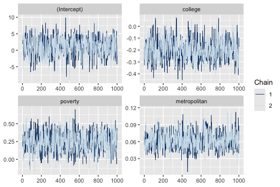
One can present the traceplot of the MCMC chain using the bayesplot::mcmc_trace function.
if (require(bayesplot)) {
  bayesplot::mcmc_trace(TPSC_model, pars = c("(Intercept)",
                                             "college",
                                             "poverty",
                                             "metropolitan"))
}
#> Loading required package: bayesplot
#> Warning: package 'bayesplot' was built under R version 4.3.1
#> This is bayesplot version 1.11.1
#> - Online documentation and vignettes at mc-stan.org/bayesplot
#> - bayesplot theme set to bayesplot::theme_default()
#>    * Does _not_ affect other ggplot2 plots
#>    * See ?bayesplot_theme_set for details on theme setting

The summary of posterior predictive distribution can be assessed using the following command. Here ystar[1] represents the posterior prediction of the first observation in the dataset, and so on.
summary(posterior::subset_draws(TPSC_model, variable = "ystar"))
#> # A tibble: 51 × 10
#>    variable   mean median    sd   mad     q5   q95  rhat ess_bulk ess_tail
#>    <chr>     <dbl>  <dbl> <dbl> <dbl>  <dbl> <dbl> <dbl>    <dbl>    <dbl>
#>  1 ystar[1]   7.25   6.20 15.3   2.03  3.28  13.4   1.00    1791.    1717.
#>  2 ystar[2]   2.67   1.35 12.6   2.02 -1.55   9.87  1.00    2016.    1885.
#>  3 ystar[3]   7.12   6.06  7.78  1.90  3.36  12.7   1.00    1691.    2043.
#>  4 ystar[4]   6.62   5.54 11.3   2.36  2.24  12.5   1.00    1688.    1793.
#>  5 ystar[5]   7.37   6.20  8.39  1.96  3.36  13.6   1.00    1811.    1809.
#>  6 ystar[6]   3.85   2.71  6.18  2.09 -0.315 11.1   1.00    1937.    1937.
#>  7 ystar[7]   5.22   3.86 14.0   2.04  0.856 12.4   1.00    1475.    1937.
#>  8 ystar[8]   5.79   4.91  5.04  1.80  2.16  11.7   1.00    1891.    1478.
#>  9 ystar[9]   6.72   5.28 17.6   2.61  1.18  14.4   1.00    1422.    1693.
#> 10 ystar[10]  7.75   6.41 10.4   1.94  3.58  14.7   1.00    2065.    1687.
#> # ℹ 41 more rows
Further comparisons between mean, median, and modal regression can be found in Section 2 of Liu, Q., Huang, X., & Bai, R. (2024) and Section 6 of Liu, Q., Huang, X., & Zhou, H. (2024).