r-KSD

Goodness-of-Fit Tests using Kernelized Stein Discrepancy.

KSD

Overview

This package provides a goodness-of-fit test of whether a given i.i.d. sample {x_i} is drawn from a given distribution. It works for any distribution once its score function (the derivative of log-density) ∇_xlog p(x) can be provided. This method is based on ``A Kernelized Stein Discrepancy for Goodness-of-fit Tests and Model Evaluation’’ by Liu, Lee, and Jordan, available at \<arXiv:1602.03253\>.

Main Components

KSD

The main function of this package is KSD, which estimates Kernelized Stein Discrepancy. Parameters include :

• x Sample of size Num_Instance x Num_Dimension
• score_function Score funtion (∇_xlog p(x)) : takes x as input and output a column vector of size Num_Instance X Dimension. User may use pryr package to pass in a function that only takes in dataset as parameter, or user may also pass in computed score for a given dataset.
• kernel Type of kernel (default = ‘rbf’)
• width Bandwidth of the kernel
• nboot Bootstrap sample size

Examples and Demos

Other methods are also in this package, including various demos and examples.

KSD requires user to provide a score function to be used for computation. For example usage and exploration, a gmm class is provided in the package, which allow test KSD using gaussian mixture model.

Consider the following examples :

1. We define a gmm, generate random data using the model, and test the null hypothesis that the data comes from the model. Obviously, the result will depend on the model and the amount of added random noise.

# Pass in a dataset generated by Gaussian distribution,
# pass in computed score rather than score function

library(KSD)
library(pryr)

model <- gmm()
X <- rgmm(model, n=100)
score_function = scorefunctiongmm(model=model, X=X)
result <- KSD(X,score_function=score_function)
result$p
#> [1] 0.899

1. We follow similar pattern, but in this example, we use pryr library to define a score function like a function handle in matlab, in which we pass in model as part of the function.

# Pass in a dataset generated by Gaussian distribution,
# use pryr package to pass in score function
library(KSD)
library(pryr)
model <- gmm()
X <- rgmm(model, n=100)
score_function = pryr::partial(scorefunctiongmm, model=model)
result <- KSD(X,score_function=score_function)
result$p
#> [1] 0.899

Demos

Premade demos include the following (Note that these demos require additional libraries)

demo_iris()
demo_normal_performance()
demo_simple_gaussian()
demo_simple_gamma()
demo_gmm()
demo_gmm_multi()

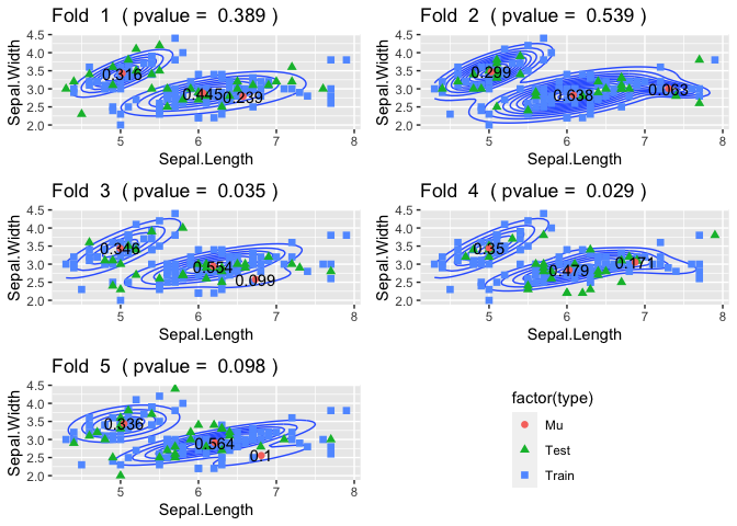
A sample run of demo_iris :

library(KSD)
library(datasets)
library(ggplot2)
library(gridExtra)
library(mclust)
library(pryr)

demo_iris()
#> [1] "Fitting GMM with 3 clusters"
#> fitting ...
#>   |                                                                                                                           |                                                                                                                   |   0%  |                                                                                                                           |========                                                                                                           |   7%  |                                                                                                                           |===============                                                                                                    |  13%  |                                                                                                                           |=======================                                                                                            |  20%  |                                                                                                                           |===============================                                                                                    |  27%  |                                                                                                                           |======================================                                                                             |  33%  |                                                                                                                           |==============================================                                                                     |  40%  |                                                                                                                           |======================================================                                                             |  47%  |                                                                                                                           |=============================================================                                                      |  53%  |                                                                                                                           |=====================================================================                                              |  60%  |                                                                                                                           |=============================================================================                                      |  67%  |                                                                                                                           |====================================================================================                               |  73%  |                                                                                                                           |============================================================================================                       |  80%  |                                                                                                                           |====================================================================================================               |  87%  |                                                                                                                           |===========================================================================================================        |  93%  |                                                                                                                           |===================================================================================================================| 100%
#> fitting ...
#>   |                                                                                                                           |                                                                                                                   |   0%  |                                                                                                                           |========                                                                                                           |   7%  |                                                                                                                           |===============                                                                                                    |  13%  |                                                                                                                           |=======================                                                                                            |  20%  |                                                                                                                           |===============================                                                                                    |  27%  |                                                                                                                           |======================================                                                                             |  33%  |                                                                                                                           |==============================================                                                                     |  40%  |                                                                                                                           |======================================================                                                             |  47%  |                                                                                                                           |=============================================================                                                      |  53%  |                                                                                                                           |=====================================================================                                              |  60%  |                                                                                                                           |=============================================================================                                      |  67%  |                                                                                                                           |====================================================================================                               |  73%  |                                                                                                                           |============================================================================================                       |  80%  |                                                                                                                           |====================================================================================================               |  87%  |                                                                                                                           |===========================================================================================================        |  93%  |                                                                                                                           |===================================================================================================================| 100%
#> fitting ...
#>   |                                                                                                                           |                                                                                                                   |   0%  |                                                                                                                           |========                                                                                                           |   7%  |                                                                                                                           |===============                                                                                                    |  13%  |                                                                                                                           |=======================                                                                                            |  20%  |                                                                                                                           |===============================                                                                                    |  27%  |                                                                                                                           |======================================                                                                             |  33%  |                                                                                                                           |==============================================                                                                     |  40%  |                                                                                                                           |======================================================                                                             |  47%  |                                                                                                                           |=============================================================                                                      |  53%  |                                                                                                                           |=====================================================================                                              |  60%  |                                                                                                                           |=============================================================================                                      |  67%  |                                                                                                                           |====================================================================================                               |  73%  |                                                                                                                           |============================================================================================                       |  80%  |                                                                                                                           |====================================================================================================               |  87%  |                                                                                                                           |===========================================================================================================        |  93%  |                                                                                                                           |===================================================================================================================| 100%
#> fitting ...
#>   |                                                                                                                           |                                                                                                                   |   0%  |                                                                                                                           |========                                                                                                           |   7%  |                                                                                                                           |===============                                                                                                    |  13%  |                                                                                                                           |=======================                                                                                            |  20%  |                                                                                                                           |===============================                                                                                    |  27%  |                                                                                                                           |======================================                                                                             |  33%  |                                                                                                                           |==============================================                                                                     |  40%  |                                                                                                                           |======================================================                                                             |  47%  |                                                                                                                           |=============================================================                                                      |  53%  |                                                                                                                           |=====================================================================                                              |  60%  |                                                                                                                           |=============================================================================                                      |  67%  |                                                                                                                           |====================================================================================                               |  73%  |                                                                                                                           |============================================================================================                       |  80%  |                                                                                                                           |====================================================================================================               |  87%  |                                                                                                                           |===========================================================================================================        |  93%  |                                                                                                                           |===================================================================================================================| 100%
#> fitting ...
#>   |                                                                                                                           |                                                                                                                   |   0%  |                                                                                                                           |========                                                                                                           |   7%  |                                                                                                                           |===============                                                                                                    |  13%  |                                                                                                                           |=======================                                                                                            |  20%  |                                                                                                                           |===============================                                                                                    |  27%  |                                                                                                                           |======================================                                                                             |  33%  |                                                                                                                           |==============================================                                                                     |  40%  |                                                                                                                           |======================================================                                                             |  47%  |                                                                                                                           |=============================================================                                                      |  53%  |                                                                                                                           |=====================================================================                                              |  60%  |                                                                                                                           |=============================================================================                                      |  67%  |                                                                                                                           |====================================================================================                               |  73%  |                                                                                                                           |============================================================================================                       |  80%  |                                                                                                                           |====================================================================================================               |  87%  |                                                                                                                           |===========================================================================================================        |  93%  |                                                                                                                           |===================================================================================================================| 100%
#> [1] "Average p value : 0.218"

Installation instructions

Currently, the code is available at https://github.com/MinHyung-Kang/KSD/ More download options will be available after CRAN submission.

Contact/Bug Reports

Minhyung(dot)Daniel(dot)Kang(at)gmail(dot)com.