Linear Mixed Models with Sparse Matrix Methods and Smoothing.

LMMsolver

The goal of the LMMsolver package is to fit (generalized) linear mixed models efficiently when the model structure is large or sparse. It provides tools for estimating variance components using restricted maximum likelihood (REML) and is designed for models that involve many random effects or smooth terms.

A key feature of the package is support for smoothing using P-splines. LMMsolver uses a sparse formulation (Boer 2023), which makes computations fast and memory efficient, especially for two-dimensional smoothing problems such as spatial surfaces or image-like data (Boer 2023; Carollo et al. 2024).

This makes LMMsolver particularly useful for applications involving spatial or temporal smoothing, large data sets, and models where standard mixed model tools become slow or impractical.

Installation

• Install from CRAN:

install.packages("LMMsolver")

• Install latest development version from GitHub (requires remotes package):

remotes::install_github("Biometris/LMMsolver", ref = "develop", dependencies = TRUE)

Example

As an example of the functionality of the package we use the USprecip data set in the spam package (Furrer and Sain 2010).

library(LMMsolver)
library(ggplot2)

## Get precipitation data from spam
data(USprecip, package = "spam")

## Only use observed data.
USprecip <- as.data.frame(USprecip)
USprecip <- USprecip[USprecip$infill == 1, ]
head(USprecip[, c(1, 2, 4)], 3)
#>      lon   lat  anomaly
#> 6 -85.95 32.95 -0.84035
#> 7 -85.87 32.98 -0.65922
#> 9 -88.28 33.23 -0.28018

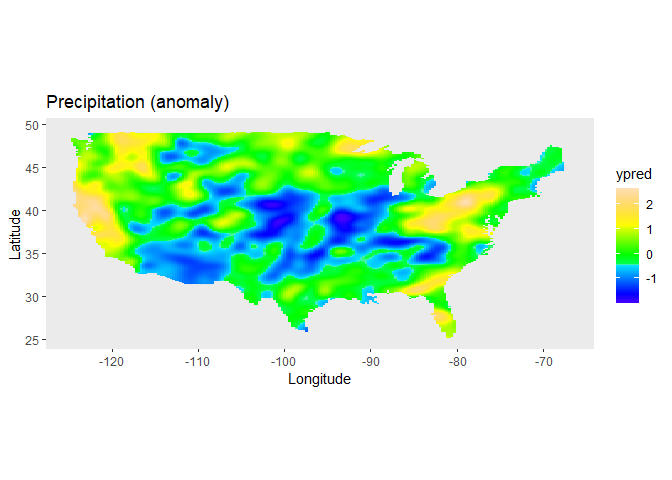
A two-dimensional P-spline can be defined with the spl2D() function, with longitude and latitude as covariates, and anomaly (standardized monthly total precipitation) as response variable:

obj1 <- LMMsolve(fixed = anomaly ~ 1,
                 spline = ~spl2D(x1 = lon, x2 = lat, nseg = c(41, 41)),
                 data = USprecip)

The spatial trend for the precipitation can now be plotted on the map of the USA, using the predict function of LMMsolver:

lon_range <- range(USprecip$lon)
lat_range <- range(USprecip$lat)
newdat <- expand.grid(lon = seq(lon_range[1], lon_range[2], length = 200),
                      lat = seq(lat_range[1], lat_range[2], length = 300))
plotDat <- predict(obj1, newdata = newdat)

plotDat <- sf::st_as_sf(plotDat, coords = c("lon", "lat"))
usa <- sf::st_as_sf(maps::map("usa", regions = "main", plot = FALSE))
sf::st_crs(usa) <- sf::st_crs(plotDat)
intersection <- sf::st_intersects(plotDat, usa)
plotDat <- plotDat[!is.na(as.numeric(intersection)), ]

ggplot(usa) + 
  geom_sf(color = NA) +
  geom_tile(data = plotDat, 
            mapping = aes(geometry = geometry, fill = ypred), 
            linewidth = 0,
            stat = "sf_coordinates") +
  scale_fill_gradientn(colors = topo.colors(100))+
  labs(title = "Precipitation (anomaly)", 
       x = "Longitude", y = "Latitude") +
  coord_sf() +
  theme(panel.grid = element_blank())

Further examples can be found in the vignette.

vignette("Solving_Linear_Mixed_Models")

References

Boer, Martin P. 2023. “Tensor Product P-Splines Using a Sparse Mixed Model Formulation.” Statistical Modelling 23 (5-6): 465–79. https://doi.org/10.1177/1471082X231178591.
Carollo, Angela, Paul Eilers, Hein Putter, and Jutta Gampe. 2024. “Smooth Hazards with Multiple Time Scales.” Statistics in Medicine. https://doi.org/10.1002/sim.10297.
Furrer, R, and SR Sain. 2010. “spam: A sparse matrix R package with emphasis on MCMC methods for Gaussian Markov random fields.” J. Stat. Softw.https://doi.org/10.18637/jss.v036.i10.