Description
Survival Prediction with Multi-Task Logistic Regression.
Description
An implementation of Multi-Task Logistic Regression (MTLR) for R. This package is based on the method proposed by Yu et al. (2011) which utilized MTLR for generating individual survival curves by learning feature weights which vary across time. This model was further extended to account for left and interval censored data.
README.md
MTLR
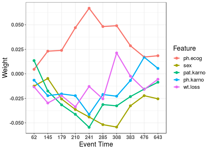
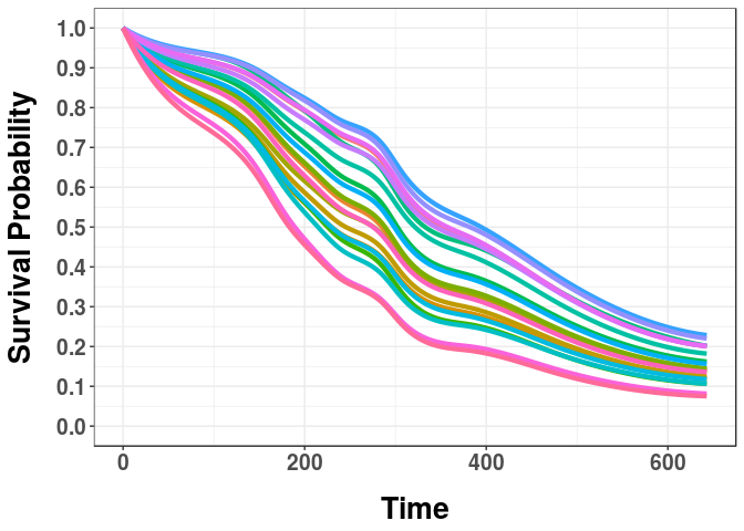
The goal of MTLR is to provide an R implementation for Multi-Task Logistic Regression. In addition to supplying the model provided by Yu et al. we have extended the model for left censoring, interval censoring, and a mixture of censoring types. Functionality includes training an MTLR model, predicting survival curves for new observations, and plotting these survival curves and feature weights estimated by MTLR.
Installation
You can install the version from CRAN or the development version from GitHub:
# CRAN:
install.packages("MTLR")

# GitHub:
# install.packages("devtools")
devtools::install_github("haiderstats/MTLR")
Example
Given a survival dataset containing event time and event status indicator (censored/uncensored) we can produce an MTLR model. For example, consider the lung dataset from the survival package:
# Load survival for the lung dataset and the Surv() function.
library(survival)
#Here we will use 9 intervals (10 time points) just for plotting purposes.
#The default is sqrt the number of observations.
mod <- mtlr(Surv(time,status)~., data = lung, nintervals = 9)
print(mod)
#>
#> Call:  mtlr(formula = Surv(time, status) ~ ., data = lung, nintervals = 9)
#>
#> Time points:
#>  [1]  62.3 145.4 179.3 210.4 241.4 284.5 308.2 383.5 476.3 642.8
#>
#>
#> Weights:
#>           Bias      inst      age      sex ph.ecog ph.karno pat.karno meal.cal  wt.loss
#> 62.27   0.1147 -0.017981  0.04891 -0.01249 0.00461 -0.00648   0.01352 -0.02617 -0.01325
#> 145.36  0.1362 -0.021147  0.03275 -0.00473 0.02312 -0.02227  -0.01753 -0.01105 -0.02974
#> 179.27  0.2119 -0.008203  0.02260 -0.02564 0.02394 -0.02046  -0.03161 -0.02310 -0.02218
#> 210.36  0.0398  0.000359  0.00816 -0.03638 0.04704 -0.02230  -0.04129 -0.01410 -0.03367
#> 241.36 -0.0996  0.009570 -0.01581 -0.04405 0.06690 -0.04139  -0.05453 -0.00808 -0.01288
#> 284.55 -0.2299  0.004869 -0.00476 -0.05180 0.04824 -0.02107  -0.03135  0.00237 -0.02552
#> 308.18 -0.3012 -0.007743 -0.00467 -0.05426 0.04908 -0.02280  -0.03264 -0.01608  0.02130
#> 383.45 -0.0289 -0.019985 -0.01030 -0.03263 0.02868 -0.00680  -0.02321 -0.01458 -0.00235
#> 476.27 -0.1285 -0.010232  0.00106 -0.02226 0.01715  0.01699  -0.01555 -0.02112 -0.01587
#> 642.82 -0.3513 -0.014975  0.02291 -0.02548 0.01847  0.00556  -0.00856  0.00373 -0.00552
#Plot feature weights:
plot(mod)

#Get survival curves for the lung dataset:
curves <- predict(mod)
#Plot the first 20 survival curves:
plotcurves(curves, 1:20)
