Tools for Multilayer and Single Layer Network Modeling.

MixMashNet

MixMashNet is an R package for estimating and analyzing Mixed Graphical Model (MGM) networks.
As the name suggests, the idea is to “mix and mash” different types of variables (continuous, categorical, binary) and even different layers of information (e.g., biomarkers, chronic diseases) to build networks that are both flexible and interpretable.

With MixMashNet you can:

• estimate single-layer networks or more complex multilayer networks
• compute centrality and bridge centrality indices
• assess community stability via non-parametric bootstrap
• obtain quantile regions for node metrics and edge weights
• visualize and explore the resulting networks interactively

In short: a bit of mix, a bit of mash, and you’re ready to build your network!

To cite the package:

De Martino, M., Triolo, F., Perigord, A., Margherita Ornago, A., Liborio Vetrano, D., and Gregorio, C., “MixMashNet: An R Package for Single and Multilayer Networks”, arXiv e-prints, Art. no. arXiv:2602.05716, 2026. doi:10.48550/arXiv.2602.05716.

Additional information and the companion interactive visualization apps can be found at the package’s website: https://arcbiostat.github.io/MixMashNet/

Installation

You can install the development version of MixMashNet from GitHub with:

# install.packages("devtools")
devtools::install_github("ARCbiostat/MixMashNet")

Example

Here we demonstrate how to estimate a single-layer MGM and assess its stability.

Preparation

Load package and example data

library(MixMashNet)
data(nhgh_data) # example dataset bundled with the package

Parallel execution (optional)

To speed up bootstrap replications we can enable parallelism with the future framework. Using multisession works on Windows, macOS, and Linux.

library(future)
library(future.apply)
#> Warning: package 'future.apply' was built under R version 4.5.2

# Use separate R sessions (cross-platform, safe in RStudio)
plan(multisession, workers = max(1, parallel::detectCores() - 1))

# When finished, you can reset with:
# plan(sequential)

Run MixMashNet

We now fit the MGM model.
Here, covariates (age, sex, re) are included in the estimation to adjust the network, but they are excluded from the visualization and centrality metrics.

fit0 <- mixMN(
  data               = nhgh_data,
  reps               = 0,                # no bootstrap: just estimate the network
  lambdaSel          = "EBIC",
  seed_model         = 42,
  cluster_method     = "louvain",
  covariates         = c("age", "sex", "re")  # adjust by covariates, exclude them from the graph
)

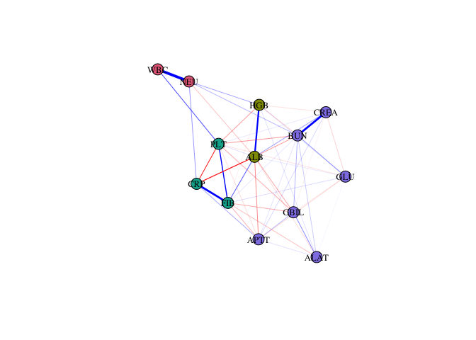
Quick visualization

Nodes are colored according to their community membership.

set.seed(2)
plot(fit0)

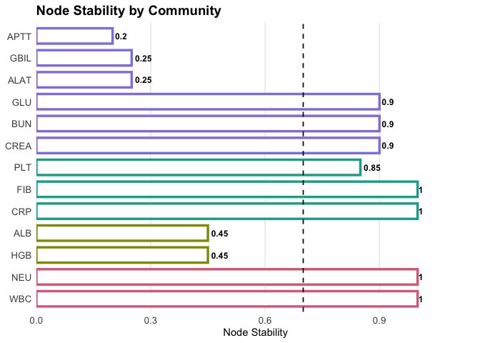
Node stability

To assess the robustness of community assignment, we re-estimate the model with non-parametric bootstrap.

fit1 <- mixMN(
  data               = nhgh_data,
  reps               = 20,             # increase reps for more stable results
  lambdaSel          = "EBIC",
  seed_model         = 42,
  seed_boot          = 42,
  cluster_method     = "infomap",
  covariates         = c("age", "sex", "re")
)
#> Total computation time: 20.4 seconds (~ 0.34 minutes).

Plot item stability:

plot(fit1, what = "stability")

Excluding unstable nodes

Nodes with stability < 0.70 are retained in the network but excluded from the clustering (they will appear in grey). Singletons are also excluded from communities.

stab1 <- membershipStab(fit1)
low_stability <- names(stab1$membership.stability$empirical.dimensions)[
    stab1$membership.stability$empirical.dimensions < 0.70
  ]

fit2 <- mixMN(
  data                 = nhgh_data,
  reps                 = 20,                    
  lambdaSel            = "EBIC",
  seed_model           = 42,
  seed_boot            = 42,
  cluster_method       = "infomap",
  covariates           = c("age", "sex", "re"),
  exclude_from_cluster = low_stability,           #exclude unstable nodes
  treat_singletons_as_excluded = TRUE             # declare not to consider singletons as communities
)
#> Total computation time: 7.8 seconds (~ 0.13 minutes).

Recompute stability:

plot(fit2, what = "stability")

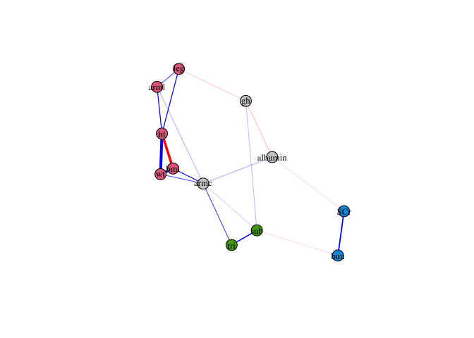
Visualization with excluded nodes

Finally, plot the updated network. Excluded nodes (unstable or singletons) are displayed in grey.

set.seed(2)
plot(fit2)

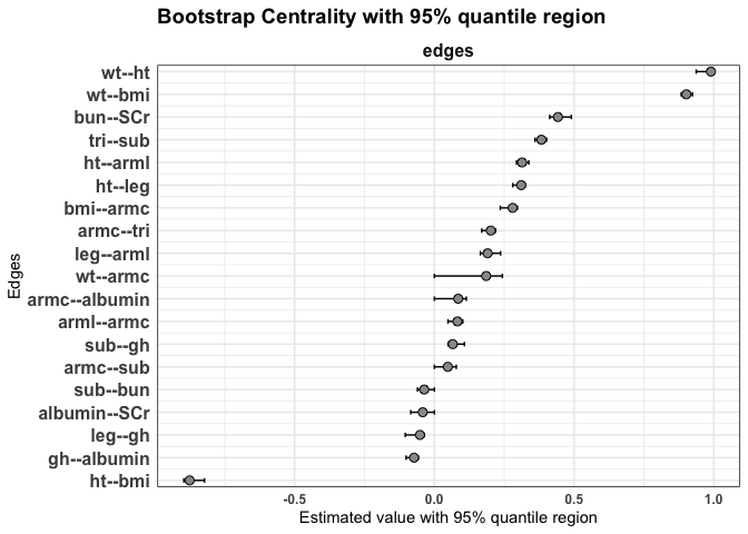
Edge weights

We can compute the edge weights with their 95% quantile regions.

plot(fit2, statistics = "edges")

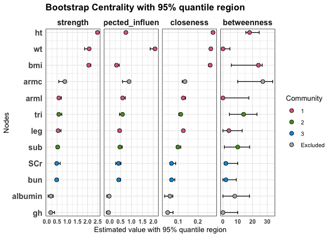
General centrality indices

We can compute standard node centrality indices (strength, expected influence, closeness, and betweenness) together with their 95% quantile regions.

plot(fit2,
  statistics = c("strength", "expected_influence", "closeness", "betweenness")
)

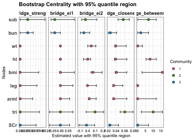
Bridge centrality indices

Bridge centrality indices quantify the role of each node as a connector between different communities. Here we display bridge strength, bridge expected influence (EI1 and EI2), bridge closeness, and bridge betweenness, with their 95% quantile regions.

plot(
  fit2,
  statistics = c("bridge_strength", "bridge_ei1", "bridge_ei2", "bridge_closeness", "bridge_betweenness")
)

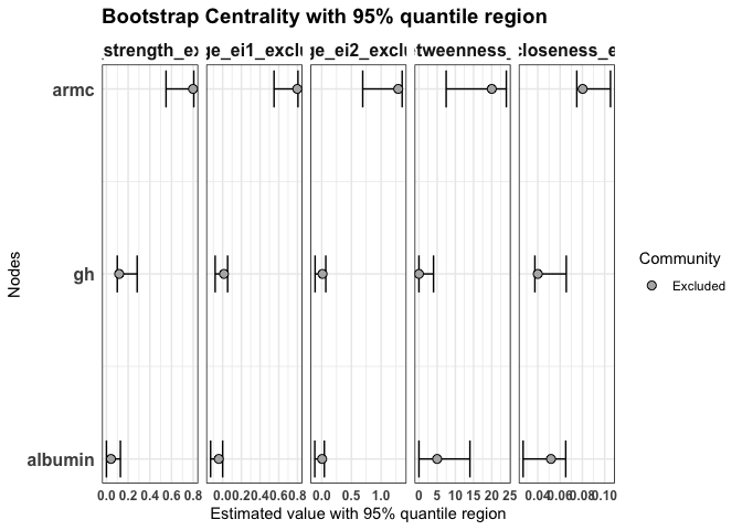
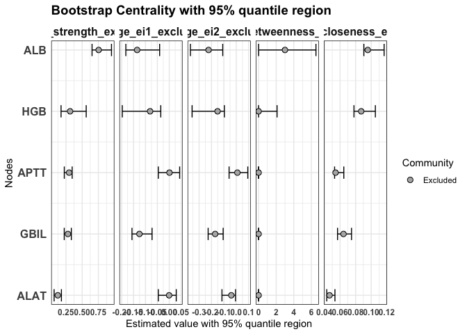
Bridge centrality indices for excluded nodes

Nodes that were excluded from clustering (e.g. due to low item stability) can also be evaluated with bridge centrality indices. This allows us to investigate their potential role in connecting existing communities, even if they are not assigned to one.

plot(
  fit2,
  statistics = c("bridge_strength_excluded", "bridge_ei1_excluded", "bridge_ei2_excluded",
              "bridge_betweenness_excluded", "bridge_closeness_excluded")
)

✨ That’s it! With just a few lines of code, you can mix, mash, and explore your networks.