Predict Cancer Subtypes Based on TCGA Data using Machine Learning Method.

OncoSubtype

Provide functionality for cancer subtyping using existing published methods or machine learning based on TCGA data.

Currently support mRNA subtyping:

• LUSC using nearest centroids method or random forest method by training TCGA data.
• LUAD using nearest centroids method or random forest method by training TCGA data.
• HNSC using nearest centroids method or random forest method by training TCGA data.
• BLCA using random forest (rf) method by training TCGA data.
• ESCA using random forest (rf) method by training TCGA data.
• ESCC using random forest (rf) method by training TCGA data.
• BRCA using PAM50 method based on R package genefu.
• STAD using random forest (rf) method by training TCGA data.

Latest release

1.0.0

Installation

You can install the released version through:

install.packages("OncoSubtype")

Example

This is a basic example for predicting the subtypes for Lung Squamous Cell Carcinoma (LUSC).

Predict LUSC mRNA Expression Subtypes using nearest centroids method

library(OncoSubtype)
library(tidyverse)
data <- get_median_centered(example_fpkm)
data <- assays(data)$centered
rownames(data) <- rowData(example_fpkm)$external_gene_name
# use default wilkerson's method
output1 <- centroids_subtype(data, disease = 'LUSC')
table(output1@subtypes)
#> 
#>     basal classical primitive secretory 
#>        44        65        26        44

Using random forest model by training TCGA LUSC data

output2 <- ml_subtype(data, disease = 'LUSC', method = 'rf', seed = 123)
table(output2@subtypes)
#> 
#>     basal classical primitive secretory 
#>        43        65        27        44

Check the consistance between two methods

confusionMatrix(as.factor(tolower(output1@subtypes)),
                as.factor(tolower(output2@subtypes)))
#> Confusion Matrix and Statistics
#> 
#>            Reference
#> Prediction  basal classical primitive secretory
#>   basal        43         1         0         0
#>   classical     0        64         1         0
#>   primitive     0         0        26         0
#>   secretory     0         0         0        44
#> 
#> Overall Statistics
#>                                           
#>                Accuracy : 0.9888          
#>                  95% CI : (0.9602, 0.9986)
#>     No Information Rate : 0.3631          
#>     P-Value [Acc > NIR] : < 2.2e-16       
#>                                           
#>                   Kappa : 0.9846          
#>                                           
#>  Mcnemar's Test P-Value : NA              
#> 
#> Statistics by Class:
#> 
#>                      Class: basal Class: classical Class: primitive
#> Sensitivity                1.0000           0.9846           0.9630
#> Specificity                0.9926           0.9912           1.0000
#> Pos Pred Value             0.9773           0.9846           1.0000
#> Neg Pred Value             1.0000           0.9912           0.9935
#> Prevalence                 0.2402           0.3631           0.1508
#> Detection Rate             0.2402           0.3575           0.1453
#> Detection Prevalence       0.2458           0.3631           0.1453
#> Balanced Accuracy          0.9963           0.9879           0.9815
#>                      Class: secretory
#> Sensitivity                    1.0000
#> Specificity                    1.0000
#> Pos Pred Value                 1.0000
#> Neg Pred Value                 1.0000
#> Prevalence                     0.2458
#> Detection Rate                 0.2458
#> Detection Prevalence           0.2458
#> Balanced Accuracy              1.0000

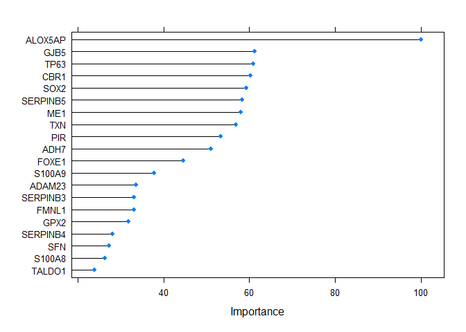
Plot important genes

vi <- varImp(output2@method, scale = TRUE)
plot(vi, top = 20) 

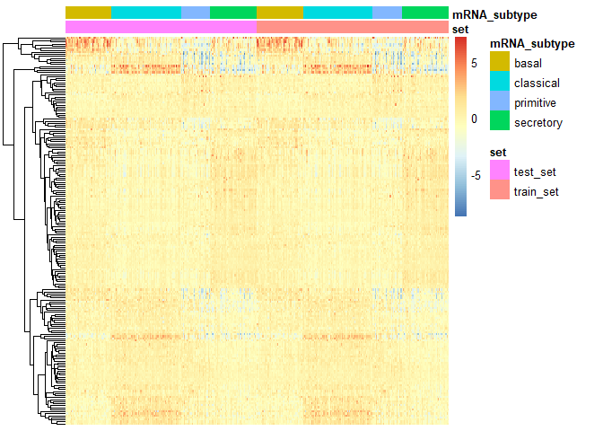
Plotheat map

PlotHeat(object = output2, set = 'both', fontsize = 10,
        show_rownames = FALSE, show_colnames = FALSE)

Report bugs or issues at here.