Description
Fast Analysis of ROC Curves.
Description
A toolkit for analyzing classifier performance by using receiver operating characteristic (ROC) curves. Performance may be assessed on a single classifier or multiple ones simultaneously, making it suitable for comparisons. In addition, different metrics allow the evaluation of local performance when working within restricted ranges of sensitivity and specificity. For details on the different implementations, see McClish D. K. (1989) <doi:10.1177/0272989X8900900307>, Vivo J.-M., Franco M. and Vicari D. (2018) <doi:10.1007/S11634-017-0295-9>, Jiang Y., et al (1996) <doi:10.1148/radiology.201.3.8939225>, Franco M. and Vivo J.-M. (2021) <doi:10.3390/math9212826> and Carrington, André M., et al (2020) <doi: 10.1186/s12911-019-1014-6>.
README.md
ROCnGO
Overview
ROCnGO provides a set of tools to study a classifier performance by using ROC curve based analysis. Package may address tasks in these type of analysis such as:
- Evaluating global classifier performance.
- Evaluating local classifier performance when a high specificity or sensitivity is required, by using different indexes that provide:
- Better interpretation of local performance.
- Better power of discrimination between classifiers with similar performance.
- Evaluating performance on several classifier simultaneously.
- Plot whole, or specific regions, of ROC curves.
Installation
install.packages("ROCnGO")
Alternatively, development version of ROCnGO can be installed from its GitHub repository with:
# install.packages("devtools")
devtools::install_github("pabloPNC/ROCnGO")
Usage
library(ROCnGO)

# Iris subset
iris_subset <- iris[iris$Species != "versicolor", ]

# Select Species = "virginica" as the condition of interest
iris_subset$Species <- relevel(iris_subset$Species, "virginica")

# Summarize a predictor over high sensitivity region
summarize_predictor(
  iris_subset,
  predictor = Sepal.Length,
  response = Species,
  threshold = 0.9,
  ratio = "tpr"
)
#> ℹ Upper threshold 1 already included in points.
#> • Skipping upper threshold interpolation
#> # A tibble: 1 × 5
#>     auc   pauc np_auc fp_auc curve_shape
#>   <dbl>  <dbl>  <dbl>  <dbl> <chr>
#> 1 0.985 0.0847  0.847  0.852 Concave
# Summarize several predictors simultaneously
summarize_dataset(
  iris_subset,
  predictors = c(Sepal.Length, Sepal.Width, Petal.Length, Petal.Width),
  response = Species,
  threshold = 0.9,
  ratio = "tpr"
)
#> ℹ Lower 0.9 and upper 1 thresholds already included in points
#> • Skipping lower and upper threshold interpolation
#> $data
#> # A tibble: 4 × 6
#>   identifier     auc   pauc np_auc fp_auc curve_shape
#>   <chr>        <dbl>  <dbl>  <dbl>  <dbl> <chr>
#> 1 Sepal.Length 0.985 0.0847 0.847   0.852 Concave
#> 2 Sepal.Width  0.166 0.0016 0.0160  0.9   Hook under chance
#> 3 Petal.Length 1     0.1    1       1     Concave
#> 4 Petal.Width  1     0.1    1       1     Concave
#>
#> $curve_shape
#> # A tibble: 2 × 2
#>   curve_shape       count
#>   <chr>             <int>
#> 1 Concave               3
#> 2 Hook under chance     1
#>
#> $auc
#> # A tibble: 2 × 3
#> # Groups:   auc > 0.5 [2]
#>   `auc > 0.5` `auc > 0.8` count
#>   <lgl>       <lgl>       <int>
#> 1 FALSE       FALSE           1
#> 2 TRUE        TRUE            3
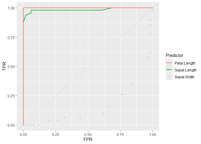
# Plot ROC curve of classifiers
plot_roc_curve(iris_subset, predictor = Sepal.Length, response = Species) +
  add_roc_curve(iris_subset, predictor = Petal.Length, response = Species) +
  add_roc_points(iris_subset, predictor = Sepal.Width, response = Species) +
  add_chance_line()