Structural Bayesian Information Criterion for Graphical Models.
SBIC: Structural Bayesian Information Criterion (SBIC) for model selection in candidate models
R-package implementation for the method presented in the paper “Information Enhanced Model Selection for Gaussian Graphical Model with Application to Metabolomic Data” by Zhou et al. 2020.
Abstract
In light of the low signal-to-noise nature of many large biological data sets, we propose a novel method to learn the structure of association networks using a Gaussian graphical model combined with prior knowledge. Our strategy includes two parts. In the rst part, we propose a model selection criterion called structural Bayesian information criterion (SBIC), in which the prior structure is modeled and incorporated into the Bayesian information criterion (BIC). It is shown that the popular extended BIC (EBIC) is a special case of SBIC. In second part, we propose a two-step algorithm to construct the candidate model pool. The algorithm is data-driven and the prior structure is embedded into the candidate model automatically. Theoretical investigation shows that under some mild conditions SBIC is a consistent model selection criterion for the high-dimensional Gaussian graphical model. Simulation studies validate the superiority of the proposed algorithm over the existing ones and show the robustness to the model misspecification. Application to relative concentration data from infant feces collected from subjects enrolled in a large molecular epidemiological cohort study validates that prior knowledge on metabolic pathway involvement is a statistically signi cant factor for the conditional dependence among metabolites. Furthermore, new relationships among metabolites are identi ed through the proposed algorithm which have not been discovered by conventional pathway analysis. Some of them have been widely recognized in the literature.
Installation
The development version from GitHub with:
# install.packages("remotes")
remotes::install_github("hoenlab/SBIC")
Example
This is a basic example which shows you how to solve a common problem:
library(SBICgraph)
#>
#> Attaching package: 'SBICgraph'
#> The following object is masked from 'package:stats':
#>
#>     simulate
library(network) # for visualization
#> network: Classes for Relational Data
#> Version 1.16.1 created on 2020-10-06.
#> copyright (c) 2005, Carter T. Butts, University of California-Irvine
#>                     Mark S. Handcock, University of California -- Los Angeles
#>                     David R. Hunter, Penn State University
#>                     Martina Morris, University of Washington
#>                     Skye Bender-deMoll, University of Washington
#>  For citation information, type citation("network").
#>  Type help("network-package") to get started.
# simulate data using the incorporated simulate function
p <- 200
m1 <- 100
m2 <- 30
d <- simulate(n=100, p=p, m1=m1, m2=m2)
data<- d$data
real<- d$realnetwork
priori<- d$priornetwork
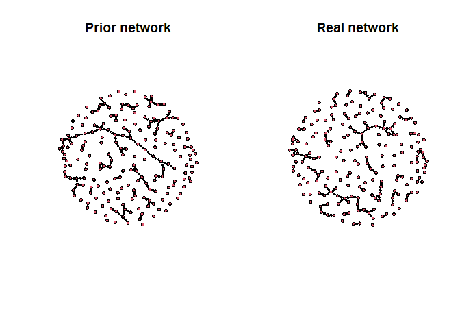
Compare between We can visualize the networks
prior_net <- network(priori)
real_net <- network(real)
par(mfrow = c(1,2))
plot(prior_net, main = "Prior network")
plot(real_net, main = "Real network")

Then we can fit SBIC using one function
lambda<- exp(seq(-10,10, length=30))
# calculating the error rate from the number of edges in the true graph and the number of discordant pairs
r1 <- m2/m1
r2 <-m2/(p*(p-1)/2-m1)
r <- (r1+r2)/2
model<- sggm(data = data, lambda = lambda, M=priori, prob = r)
Comparing the estimated network to the true and prior network. Our comparison function above calcualtes the Positive selection rate (PSR) and the False positive rate (FDR)
print("Comparing estimated model with the real network")
#> [1] "Comparing estimated model with the real network"
comparison(real = real, estimate = model$networkhat)
#> $PSR
#> [1] 0.36
#>
#> $FDR
#> [1] 0.4285714
print("Comparing the prior network with the real network")
#> [1] "Comparing the prior network with the real network"
comparison(real = real, estimate = priori)
#> $PSR
#> [1] 0.7
#>
#> $FDR
#> [1] 0.3