

Discrete Log-Gaussian Cox Processes for Aggregated Disease Counts.
SDALGCP2 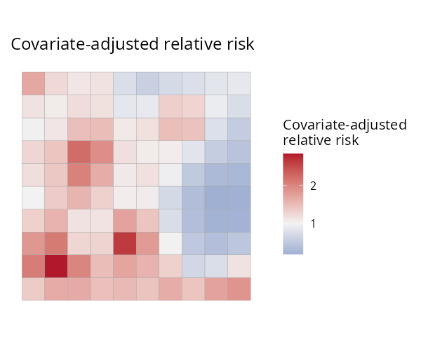


Fast, modern disease mapping. SDALGCP2 fits a spatially discrete approximation to a log-Gaussian Cox process (SDA-LGCP) to spatially aggregated disease counts, with a one-line, glm-like interface and C++ speed. The method is described in Johnson, Diggle & Giorgi (2019, Statistics in Medicine, doi:10.1002/sim.8339).
Installation
# install.packages("remotes")
remotes::install_github("olatunjijohnson/SDALGCP2")
You need a C++ toolchain (Rtools on Windows, Xcode CLT on macOS) because the performance-critical kernels are compiled.
Quick start — one line to fit
data is an sf object whose columns hold the response, covariates and offset. Everything else (candidate-point spacing, the spatial scale, MCMC settings) is chosen automatically.
library(SDALGCP2)

fit <- sdalgcp(cases ~ deprivation + offset(log(population)), data = regions)

summary(fit)              # glm-style coefficient table + spatial parameters
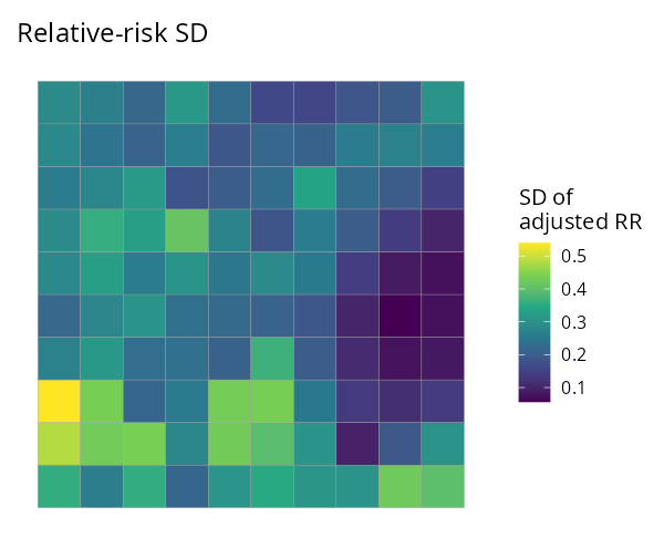
rr  <- predict(fit)       # an sf: relative_risk, relative_risk_se, adjusted_rr, adjusted_rr_se
plot(fit)                 # relative-risk map
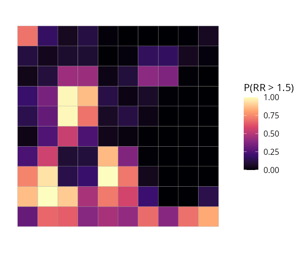
plot(fit, "exceedance", threshold = 1.5)   # hotspot probabilities
That is the whole workflow. The same sdalgcp() call also covers:
| You want… | Add… |
|---|---|
| raster (continuous) covariates | rasters = my_raster (enter on the intensity scale) |
| a spatio-temporal model | time = "year" |
| population-weighted aggregation | popden = pop_raster |
What you get
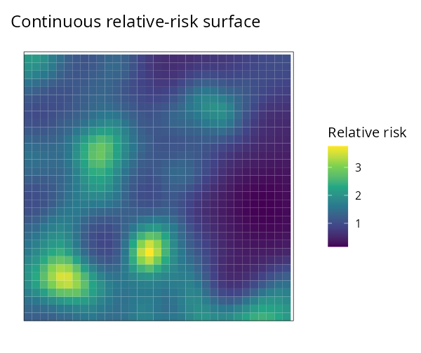
| Relative risk | Uncertainty (SD) | Exceedance P(RR > 1.5) | Continuous surface |
|---|---|---|---|
|  |  |  |
Why SDALGCP2
- Easy:
sdalgcp(formula, data)— feels likeglm(); sensible defaults so a first fit needs no tuning. - Fast: aggregated correlation assembly, the MALA sampler and the Monte Carlo likelihood run in C++ (RcppArmadillo + OpenMP) — 8–10× faster end-to-end than the original, returning the same estimates (see Performance).
- Grid-free scale: the spatial scale
φis optimised continuously by default (no grid), with a proper standard error — see the derivation PDF. - Continuous covariates done right: rasters enter on the intensity scale (log-sum-exp), not by averaging predictors over polygons — see the raster PDF.
- Spatio-temporal without ever forming the
(N·T)²covariance. - Honest uncertainty: re-anchored Monte Carlo likelihood, importance-sampling diagnostics, a nugget term, model checking (residual Moran's I).
Tutorials
See the package website for worked, reproducible articles:
- Spatial disease mapping — the full workflow end to end.
- Raster predictors — intensity-scale covariates vs naive areal averaging.
- Spatio-temporal — space-time relative risk.
- Estimating the scale — grid (
scale = "grid") vs continuous (scale = "continuous")φ.
Reference
Johnson, O., Diggle, P. & Giorgi, E. (2019). A spatially discrete approximation to log-Gaussian Cox processes for modelling aggregated disease count data. Statistics in Medicine 38, 4871–4887. \doi{10.1002/sim.8339}