Inference with Stochastic Gradient Descent.
SGDinference
SGDinference is an R package that provides estimation and inference methods for large-scale mean and quantile regression models via stochastic (sub-)gradient descent (S-subGD) algorithms. The inference procedure handles cross-sectional data sequentially:
- updating the parameter estimate with each incoming “new observation”,
- aggregating it as a Polyak-Ruppert average, and
- computing an asymptotically pivotal statistic for inference through random scaling.
The methodology used in the SGDinference package is described in detail in the following papers:
Lee, S., Liao, Y., Seo, M.H. and Shin, Y., 2022. Fast and robust online inference with stochastic gradient descent via random scaling. In Proceedings of the AAAI Conference on Artificial Intelligence (Vol. 36, No. 7, pp. 7381-7389). https://doi.org/10.1609/aaai.v36i7.20701.
Lee, S., Liao, Y., Seo, M.H. and Shin, Y., 2023. Fast Inference for Quantile Regression with Tens of Millions of Observations. arXiv:2209.14502 [econ.EM] https://doi.org/10.48550/arXiv.2209.14502.
Installation
You can install the development version from GitHub with:
# install.packages("devtools") # if you have not installed "devtools" package
devtools::install_github("SGDinference-Lab/SGDinference")
We begin by calling the SGDinference package.
library(SGDinference)
set.seed(100723)
Case Study: Estimating the Mincer Equation
To illustrate the usefulness of the package, we use a small dataset included in the package. Specifically, the Census2000 dataset from Acemoglu and Autor (2011) consists of observations on 26,120 nonwhite, female workers. This small dataset is constructed from “microwage2000_ext.dta” at https://economics.mit.edu/people/faculty/david-h-autor/data-archive. Observations are dropped if hourly wages are missing or years of education are smaller than 6. Then, a 5 percent random sample is drawn to make the dataset small. The following three variables are included:
- ln_hrwage: log hourly wages
- edyrs: years of education
- exp: years of potential experience
We now define the variables.
    y = Census2000$ln_hrwage
  edu = Census2000$edyrs
  exp = Census2000$exp
 exp2 = exp^2/100
As a benchmark, we first estimate the Mincer equation and report the point estimates and their 95% heteroskedasticity-robust confidence intervals.
mincer = lm(y ~ edu + exp + exp2)
inference = lmtest::coefci(mincer, df = Inf,
                             vcov = sandwich::vcovHC)
results = cbind(mincer$coefficients,inference)
colnames(results)[1] = "estimate"
print(results)
#>                estimate       2.5 %      97.5 %
#> (Intercept)  0.58114741  0.52705757  0.63523726
#> edu          0.12710477  0.12329983  0.13090971
#> exp          0.03108721  0.02877637  0.03339806
#> exp2        -0.04498841 -0.05070846 -0.03926835
Estimating the Mean Regression Model Using SGD
We now estimate the same model using SGD.
 mincer_sgd = sgdi_lm(y ~ edu + exp + exp2)
 print(mincer_sgd)
#> Call:
#> sgdi_lm(formula = y ~ edu + exp + exp2)
#>
#> Coefficients:
#>             Coefficient    CI.Lower    CI.Upper
#> (Intercept)  0.58714627  0.51899447  0.65529806
#> edu          0.12651235  0.12290359  0.13012112
#> exp          0.03152331  0.02788511  0.03516150
#> exp2        -0.04601193 -0.05566846 -0.03635539
#>
#> Significance Level: 95 %
It can be seen that the estimation results are similar between two methods. There is a different command that only computes the estimates but not confidence intervals.
 mincer_sgd = sgd_lm(y ~ edu + exp + exp2)
 print(mincer_sgd)
#> Call:
#> sgd_lm(formula = y ~ edu + exp + exp2)
#>
#> Coefficients:
#>             Coefficient
#> (Intercept)  0.58621823
#> edu          0.12658176
#> exp          0.03152287
#> exp2        -0.04599148
We compare the execution times between two versions and find that there is not much difference in this simple example. By construction, it takes more time to conduct inference via sgdi_lm.
library(microbenchmark)
res <- microbenchmark(sgd_lm(y ~ edu + exp + exp2),
                      sgdi_lm(y ~ edu + exp + exp2),
                      times=100L)
print(res)
#> Unit: milliseconds
#>                           expr      min       lq      mean    median        uq
#>   sgd_lm(y ~ edu + exp + exp2) 7.612649 7.783084  8.795013  7.939131  9.419628
#>  sgdi_lm(y ~ edu + exp + exp2) 9.605035 9.805727 10.646169 10.028305 10.539734
#>       max neval
#>  15.17188   100
#>  14.60316   100
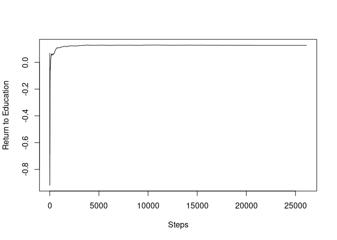
To plot the SGD path, we first construct a SGD path for the return to education coefficients.
mincer_sgd_path = sgdi_lm(y ~ edu + exp + exp2, path = TRUE, path_index = 2)
Then, we can plot the SGD path.
plot(mincer_sgd_path$path_coefficients, ylab="Return to Education", xlab="Steps", type="l")

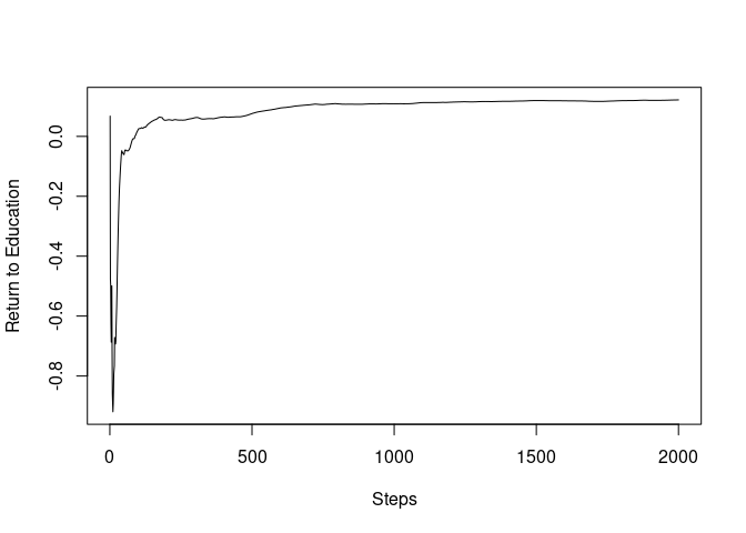
To observe the initial paths, we now truncate the paths up to 2,000.
plot(mincer_sgd_path$path_coefficients[1:2000], ylab="Return to Education", xlab="Steps", type="l")

print(c("2000th step", mincer_sgd_path$path_coefficients[2000]))
#> [1] "2000th step"       "0.121832196962998"
print(c("Final Estimate", mincer_sgd_path$coefficients[2]))
#> [1] "Final Estimate"    "0.126481851251926"
It can be seen that the SGD path almost converged only after the 2,000 steps, less than 10% of the sample size.
What else the package can do
See the vignette for the quantile regression example.
References
Acemoglu, D. and Autor, D., 2011. Skills, tasks and technologies: Implications for employment and earnings. In Handbook of labor economics (Vol. 4, pp. 1043-1171). Elsevier.
Lee, S., Liao, Y., Seo, M.H. and Shin, Y., 2022. Fast and robust online inference with stochastic gradient descent via random scaling. In Proceedings of the AAAI Conference on Artificial Intelligence (Vol. 36, No. 7, pp. 7381-7389). https://doi.org/10.1609/aaai.v36i7.20701.
Lee, S., Liao, Y., Seo, M.H. and Shin, Y., 2023. Fast Inference for Quantile Regression with Tens of Millions of Observations. arXiv:2209.14502 [econ.EM] https://doi.org/10.48550/arXiv.2209.14502.