Functions for Stochastic Search Variable Selection (SSVS).

SSVS

The goal of {SSVS} is to provide functions for performing stochastic search variable selection (SSVS) for binary and continuous outcomes and visualizing the results. SSVS is a Bayesian variable selection method used to estimate the probability that individual predictors should be included in a regression model. Using MCMC estimation, the method samples thousands of regression models in order to characterize the model uncertainty regarding both the predictor set and the regression parameters.

Installation

You can install the development version of {SSVS} from GitHub with:

# install.packages("remotes")
remotes::install_github("sabainter/SSVS")

Example 1 - continuous response variable

Consider a simple example using SSVS on the mtcars dataset to predict quarter mile times. We first specify our response variable (“qsec”), then choose our predictors and run the ssvs() function.

library(SSVS)
set.seed(1000)
outcome <- 'qsec'
predictors <- c('cyl', 'disp', 'hp', 'drat', 'wt',
 'vs', 'am', 'gear', 'carb','mpg')

results <- ssvs(data = mtcars, x = predictors, y = outcome, prior.probs = .5, progress = FALSE)

The results can be summarized and printed using the summary() function. This will display the MIP for each predictor, the average coefficients including and excluding zeros, and credible intervals for each coefficient.

summary_results <- summary(results, interval = 0.9, ordered = TRUE)

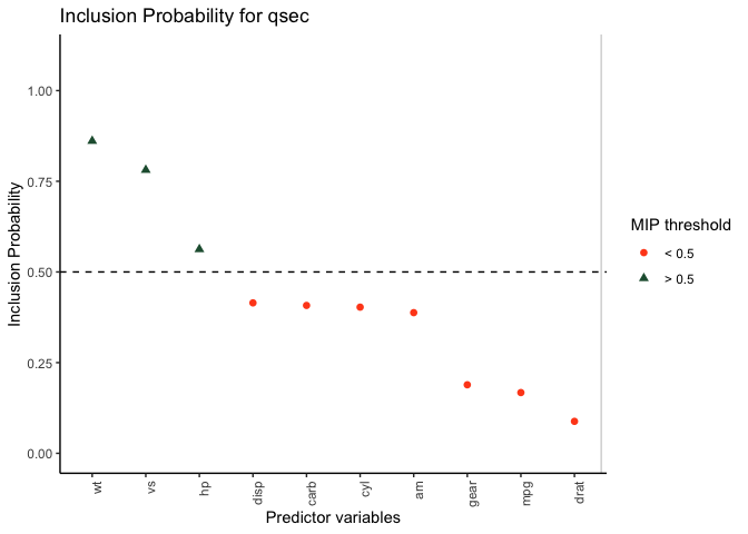
The MIPs for each predictor can then be visualized using the plot() function.

plot(results)

Example 2 - binary response variable

In the example above, the response variable was a continuous variable. The same workflow can be used for binary variables by specifying continuous = FALSE to the ssvs() function.

As an example, let’s create a binary variable:

library(AER)
#> Warning: package 'AER' was built under R version 4.5.2
data(Affairs)
Affairs$hadaffair[Affairs$affairs > 0] <- 1
Affairs$hadaffair[Affairs$affairs == 0] <- 0

Then define the outcome and predictors.

outcome <- "hadaffair"
predictors <- c("gender", "age", "yearsmarried", "children", "religiousness", "education", "occupation", "rating")

And finally run the model:

set.seed(1000)
results <- ssvs(data = Affairs, x = predictors, y = outcome, continuous = FALSE, progress = FALSE)

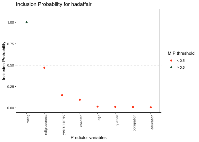
Now the results can be summarized or visualized in the same manner.

summary_results <- summary(results, interval = 0.9, ordered = TRUE)

plot(results)

Example 3 - SSVS with multiple imputation (MI)

First, we will use the mice() function from the {mice} package to perform multiple imputation.

library(mice)
#> 
#> Attaching package: 'mice'
#> The following object is masked from 'package:stats':
#> 
#>     filter
#> The following objects are masked from 'package:base':
#> 
#>     cbind, rbind

# Load the mtcars dataset
data <- mtcars

# Introduce random missingness in 10% of the data
set.seed(123)  
n <- nrow(data) * ncol(data)
missing_indices <- sample(n, size = 0.1 * n, replace = FALSE)

# Convert missing indices to row-column positions
rows <- (missing_indices - 1) %% nrow(data) + 1
cols <- (missing_indices - 1) %/% nrow(data) + 1

# Assign NA to the identified positions
for (i in seq_along(rows)) {
  data[rows[i], cols[i]] <- NA
}

# Perform multiple imputation using mice
imputed_data <- mice(data, m = 5, maxit = 50, seed = 123)

# Display the results of the imputation
summary(imputed_data)

# Extract and show the first completed dataset
imputed_mtcars <- complete(imputed_data, "long")
head(imputed_mtcars)

We will use this multiply imputed data set for SSVS, using the ssvs_mi() function.

outcome <- 'qsec'
predictors <- c('cyl', 'disp', 'hp', 'drat', 'wt', 'vs', 'am', 'gear', 'carb','mpg')
imputation <- '.imp'
results <- ssvs_mi(data = imputed_mtcars, y = outcome, x = predictors, imp = imputation)

The results of SSVS with MI can be summarized with the summary() and plot() functions. This will summarize across imputations for each predictor: the average MIP and the mean, minimum, maximum, and average nonzero beta coefficients.

Interactive version

You can launch an interactive (shiny) web application that lets you run SSVS analyses without programming. Simply install this package and run SSVS::launch() in an R console.