Process Stream Temperature, Intermittency, and Conductivity (STIC) Sensor Data.

STICr

The goal of STICr (pronounced “sticker”) is to provide a standardized set of functions for working with data from Stream Temperature, Intermittency, and Conductivity (STIC) loggers, first described in Chapin et al. (2014). STICs and other intermittency sensors are becoming more popular, but their raw data output is not in a form that allows for convenient analysis. This package aims to provide a set of functions for tidying the raw data from these loggers, as well as calibrating their conductivity measurements to specific conductivity (SpC) and classifying the conductivity data to generate a classified “wet/dry” data set.

Installation

You can install STICr from CRAN or the development version of STICr from GitHub with:

# install.packages("STICr")  # if needed: install package from CRAN
# devtools::install_github("HEAL-KGS/STICr") # if needed: install dev version from GitHub
library(STICr)

Example

This is an example workflow that shows the main functionality of the package. A more detailed version is available in the package vignette.

Step 1: Load data

# read in raw HOBO data and tidy
df_tidy <- tidy_hobo_data(infile = "https://samzipper.com/data/raw_hobo_data.csv", outfile = FALSE)
head(df_tidy)
#>              datetime condUncal  tempC
#> 1 2021-07-16 22:00:00   88178.4 27.764
#> 2 2021-07-16 22:15:00   77156.1 28.655
#> 3 2021-07-16 22:30:00   74400.5 28.060
#> 4 2021-07-16 22:45:00   74400.5 27.764
#> 5 2021-07-16 23:00:00   74400.5 27.862
#> 6 2021-07-16 23:15:00   71644.9 27.370

Step 2: Get and apply calibration

The second function is called get_calibration and is demonstrated below. The function intakes a STIC calibration data frame with columns standard and conductivity_uncaland outputs a fitted model object relating spc to the uncalibrated conductivity values measured by the STIC.

# load calibration
lm_calibration <- get_calibration(calibration_standard_data)

# apply calibration
df_calibrated <- apply_calibration(
  stic_data = df_tidy,
  calibration = lm_calibration,
  outside_std_range_flag = T
)
head(df_calibrated)
#>              datetime condUncal  tempC      SpC outside_std_range
#> 1 2021-07-16 22:00:00   88178.4 27.764 857.3845                  
#> 2 2021-07-16 22:15:00   77156.1 28.655 752.0820                  
#> 3 2021-07-16 22:30:00   74400.5 28.060 725.7561                  
#> 4 2021-07-16 22:45:00   74400.5 27.764 725.7561                  
#> 5 2021-07-16 23:00:00   74400.5 27.862 725.7561                  
#> 6 2021-07-16 23:15:00   71644.9 27.370 699.4302

Step 3: Classify data

# classify data
df_classified <- classify_wetdry(
  stic_data = df_calibrated,
  classify_var = "SpC",
  threshold = 100,
  method = "absolute"
)
head(df_classified)
#>              datetime condUncal  tempC      SpC outside_std_range wetdry
#> 1 2021-07-16 22:00:00   88178.4 27.764 857.3845                      wet
#> 2 2021-07-16 22:15:00   77156.1 28.655 752.0820                      wet
#> 3 2021-07-16 22:30:00   74400.5 28.060 725.7561                      wet
#> 4 2021-07-16 22:45:00   74400.5 27.764 725.7561                      wet
#> 5 2021-07-16 23:00:00   74400.5 27.862 725.7561                      wet
#> 6 2021-07-16 23:15:00   71644.9 27.370 699.4302                      wet

Step 4: QAQC

# apply qaqc function
df_qaqc <-
  qaqc_stic_data(
    stic_data = df_classified,
    spc_neg_correction = T,
    inspect_deviation = T,
    deviation_size = 2,
    window_size = 96
  )
head(df_qaqc)
#>              datetime condUncal  tempC      SpC wetdry QAQC
#> 1 2021-07-16 22:00:00   88178.4 27.764 857.3845    wet     
#> 2 2021-07-16 22:15:00   77156.1 28.655 752.0820    wet     
#> 3 2021-07-16 22:30:00   74400.5 28.060 725.7561    wet     
#> 4 2021-07-16 22:45:00   74400.5 27.764 725.7561    wet     
#> 5 2021-07-16 23:00:00   74400.5 27.862 725.7561    wet     
#> 6 2021-07-16 23:15:00   71644.9 27.370 699.4302    wet
table(df_qaqc$QAQC)
#> 
#>      DO   O 
#> 916   1  83

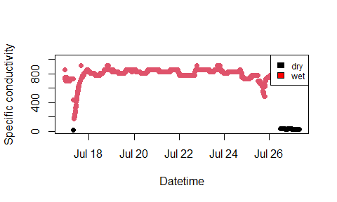
Step 5: Plot classified data

# plot SpC through time, colored by wetdry
plot(df_classified$datetime, df_classified$SpC,
  col = as.factor(df_classified$wetdry),
  pch = 16,
  lty = 2,
  xlab = "Datetime",
  ylab = "Specific conductivity"
)
legend("topright", c("dry", "wet"),
  fill = c("black", "red"), cex = 0.75
)

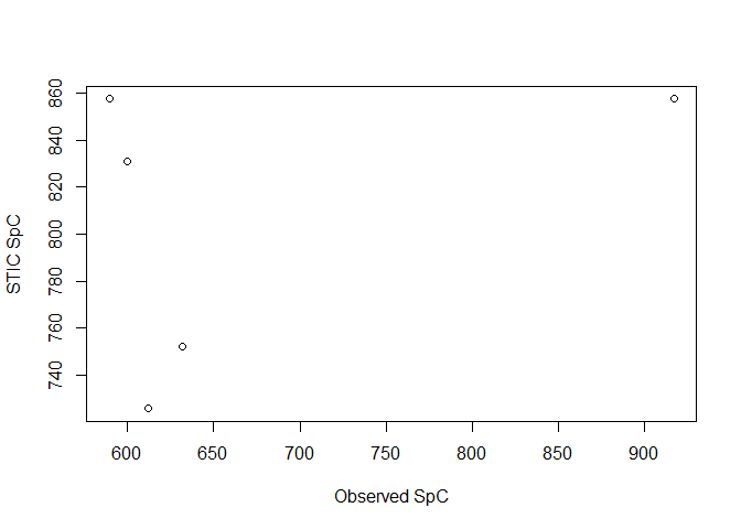
Step 6: Compare to field observations

# create validation data frame
stic_validation <-
  validate_stic_data(
    stic_data = classified_df,
    field_observations = field_obs,
    max_time_diff = 30,
    join_cols = NULL,
    get_SpC = TRUE,
    get_QAQC = FALSE
  )

# compare the field observations and classified STIC data in table
head(stic_validation)
#>              datetime wetdry_obs  SpC_obs condUncal_STIC wetdry_STIC SpC_STIC
#> 1 2021-07-16 18:03:00        wet 612.1672        74400.5         wet 725.7561
#> 2 2021-07-19 15:01:00        wet 589.4157        88178.4         wet 857.3845
#> 3 2021-07-21 02:44:00        dry 599.6622        85422.8         wet 831.0587
#> 4 2021-07-23 13:55:00        wet 916.8215        88178.4         wet 857.3845
#> 5 2021-07-25 16:27:00        wet 631.9857        77156.1         wet 752.0820
#>   timediff_min
#> 1            3
#> 2            1
#> 3           -1
#> 4           -5
#> 5           -3

# calculate percent classification accuracy
sum(stic_validation$wetdry_obs == stic_validation$wetdry_STIC) / length(stic_validation$wetdry_STIC)
#> [1] 0.8

# compare SpC as a plot
plot(stic_validation$SpC_obs, stic_validation$SpC_STIC,
  xlab = "Observed SpC", ylab = "STIC SpC"
)