Partial Least-Squares Algorithm for Categorical and Scalar Functional Data.

SmoothPLS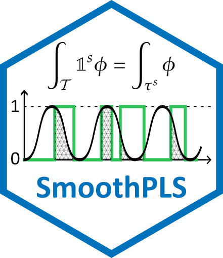

Overview

SmoothPLS is a R package designed for Hybrid Functional Data Analysis. It implements a novel approach to Functional Partial Least Squares (FPLS) by integrating categorical functional predictors through the concept of active area integration.

This work was developed as part of a PhD project at DECATHLON in collaboration with INRIA.

Key features

• SmoothPLS: integration of categorical states as indicator functions for smoother regression curves.
• Hybrid data: seamlessly handles both Scalar Functional Data (SFD) and Categorical Functional Data (CFD).
• Interpretability: provides continuous regression curves.
• Comparison suite: built-in functions to compare results with Naive (discretized) PLS and Standard Functional PLS.

Methodological background

SmoothPLS builds upon the fundamental principles of Functional PLS (FPLS) regression, specifically the approximation of functional predictors through basis expansions, as established by Aguilera, Preda et al. (2010) [1].

The primary contribution lies in modeling categorical state changes as functional indicator functions, $\mathbb{1}^s_t$. Instead of discretizing transitions, the model computes components via active area integration (illustrated in the package logo), effectively integrating basis functions over the specific intervals, $\tau_s$, where a state is active:

$$\Lambda_{s,j} = \int_{\mathcal{T}} \mathbb{1}^s_t \phi_j(t) dt = \int_{\tau_s} \phi_j(t) dt, \quad \text{with} \quad \tau_s = \lbrace t \in \mathcal{T} \mid X(t) = s\rbrace \quad \text{and} \quad \mathbb{1}_s^t = \begin{cases} 1 & \text{if } X(t) = s \ 0 & \text{otherwise} \end{cases}$$

This formulation ensures that the smoothing process respects the continuous nature of state transitions within the Functional PLS framework.

Installation

The package is currently in development. The latest stable version can be installed via:

# install.packages("devtools")
devtools::install_github("FrancoisBassac/SmoothPLS")

Documentation

The complete package documentation—including function references, detailed vignettes, and usage examples—is available online:

Explore the SmoothPLS documentation website

Documentation overview

• Reference: comprehensive manual for all functions (including smoothPLS, funcPLS, and naivePLS).
• Articles (vignettes): step-by-step tutorials, such as the comparison of PLS methods for CFD and multivariate functional data.
• Getting started: quick installation guide and basic usage.

Quick start example

The following example demonstrates how to fit and compare models, based on the single-state CFD vignette:

library(SmoothPLS)

# 1. Generate Synthetic Data
df_x <- generate_X_df(nind = 100, curve_type = 'cat')
Y_df <- generate_Y_df(df_x, curve_type = 'cat', 
                      beta_real_func_or_list = beta_1_real_func)

# 2. Fit Smooth PLS Model
basis <- create_bspline_basis(start = 0, end = 100, nbasis = 10)
spls_model <- smoothPLS(df_list = df_x, Y = Y_df$Y_noised, 
                        basis_obj = basis, curve_type_obj = 'cat')

# 3. Predict and Visualize
preds <- smoothPLS_predict(df_x, spls_model$reg_obj, curve_type = 'cat')
plot(spls_model$reg_obj$CatFD_1_state_1, main="SmoothPLS Regression Curve")

Performance tuning: parallel processing

When parallel = TRUE, SmoothPLS utilizes the future framework to parallelize the numerical integration steps (e.g., $\Lambda$ matrix evaluation).

To mitigate computational overhead on smaller datasets, the package implements dynamic load balancing. It calculates an optimal number of background workers required for the specific task to maximize efficiency.

The default threshold is set to 2500 integral evaluations per core. The engine allocates one core for every 2500 integrals (calculated as individuals $\times$ basis functions). For instance: * Under 2,500 integrals: The model executes sequentially (1 core) to avoid setup overhead. * 5,000 integrals: The engine allocates exactly 2 cores. * Large datasets (e.g., 50,000+ integrals): The engine recruits the maximum number of available cores, reserving 2 cores to maintain operating system stability.

This threshold can be manually adjusted based on specific hardware capabilities (e.g., lowered for UNIX systems with low forking overhead) by setting a global option before model execution:

# Lower the threshold to 500 evaluations per core
options(SmoothPLS.parallel_threshold = 500)

Affiliations and applications

Industrial partners

• Decathlon – Main industrial partner.
• Decathlon SportsLab – The research and development center.
• Kiprun Pacer – The training application using advanced running data:
  • Official Website
  • App Store / Play Store

Research institutions

• Inria – National Institute for Research in Digital Science and Technology.
• Inria Datavers – The research team specialized in stochastic modeling and data analysis.

Roadmap and future releases

SmoothPLS is under active development. Upcoming updates will focus on computational efficiency and the expansion of theoretical capabilities:

• [v0.1.4] Parallel processing: implementation of multicore computing to drastically reduce integration time for large datasets (e.g., thousands of Active Areas).
• [v0.1.6] Hybrid data framework: support for integrating standard non-functional covariates (e.g., user age, weight) alongside Categorical and Scalar Functional Data.
• [v0.2.0] Penalized functional regression (univariate): addition of roughness penalties to the B-spline coefficients to increase model robustness.
• [v0.2.1] Penalized functional regression (multivariate): extension of the penalized framework to the full multivariate model.

Detailed Example: One-State Categorical Functional Data

This example illustrates how SmoothPLS processes CFD by modeling transitions as functional objects. For comprehensive details, refer to the full vignette.

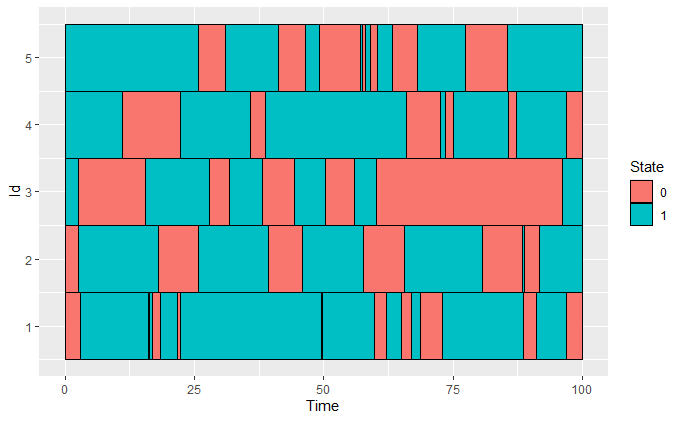
1. Data visualization

We simulate a categorical time series where individuals alternate between state 0 and state 1 over time.

library(SmoothPLS)

df_x <- generate_X_df(nind = 100, start = 0, end = 100, curve_type = 'cat')

plot_CFD_individuals(df_x, by_cfda = TRUE)

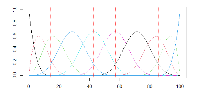
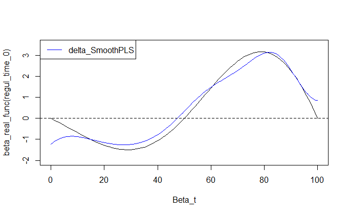
2. Model fitting and prediction

The SmoothPLS model is fitted to a response variable with added noise, $Y$, and the resulting regression curve, $\beta(t)$, is compared against the ground truth.

# Define a B-spline basis
basis <- create_bspline_basis(start = 0, end = 100, nbasis = 10)
plot(basis)

# Generate response Y linked to the time spent in state 1
Y_df <- generate_Y_df(df_x, curve_type = 'cat', 
                      beta_real_func_or_list = beta_1_real_func)

# Fit the SmoothPLS model
spls_obj <- smoothPLS(df_list = df_x, Y = Y_df$Y_noised, 
                      basis_obj = basis, curve_type_obj = 'cat',
                      print_steps = FALSE, print_nbComp = FALSE, 
                      plot_rmsep = FALSE, plot_reg_curves = FALSE)

# Extract parameters for plotting
delta <- mod_seq$reg_obj$CatFD_1_state_1
regul_time_0 <- seq(0, 100, length.out = length(delta))

y_lim = eval_max_min_y(f_list = list(beta_real_func, 
                                     delta), 
                       regul_time = regul_time_0)

plot(regul_time_0, beta_real_func(regul_time_0), type='l', xlab="Beta_t",
     ylim = c(-2, 3.5))
plot(delta, add=TRUE, col='blue')
legend("topleft",
       legend = c("delta_SmoothPLS"),
       col = c("blue"),
       lty = 1,
       lwd = 1)

References

[1] Aguilera, A. M., Escabias, M., Preda, C., & Saporta, G. (2010). "Using basis expansions for estimating functional PLS regression. Applications with chemometric data". Chemometrics and Intelligent Laboratory Systems, 104(2), 289-305. https://doi.org/10.1016/j.chemolab.2010.09.007