Sound Waves Onto Morphometric Data.

Welcome to SoundShape

Here, you will find information on how to implement a promising, and yet little explored method for biacoustical analysis: the so called eigensound analysis developed by MacLeod, Krieger and Jones (2013) and expanded by Rocha & Romano (2021).

Select your acoustic units using Raven Pro Software

Since SoundShape's version 1.3.0, the function raven.to.wave allows the creation of ".wav" files based on selections made using Raven Pro, which is commonplace in bioacoustical analysis. Topic 3 below provides information on how to do it.

Introduction on eigensound analysis

Eigensound is a multidisciplinary method focused on the direct comparison between homologous sounds from different species (i.e. stereotyped calls/acoustic units; Macleod et al., 2013; Rocha & Romano, 2021). It consists on applying a sampling grid over the representation of sound (i.e. spectrogram data; Figs. 1 and 2) and then translate the spectrogram into a dataset that can be analyzed similarly to coordinate sets used in Geometric Morphometrics Methods (GMM). By doing so, eigensound crosses the bridge between Bioacoustics and GMM.

Despite being well described by Macleod et al. (2013), the method lacked a free and open platform to run the analysis. SoundShape package was written on R platform to fill this applicability gap. The package features functions that enable anyone familiar with R to easily go from sound waves to principal components analysis (PCA), using tools extracted from traditional bioacoustics (i.e.tuneR and seewave packages), geometric morphometrics (i.e.geomorph package) and multivariate analysis (e.g.stats package).

Thanks for using SoundShape and enjoy your reading!

Note: Should you experience problems running any function, please feel free to report any issues here.

library(SoundShape)

# Sample data from SoundShape
data(cuvieri)

# Select acoustic unit from sample
cuvieri.cut <- seewave::cutw(cuvieri, f=44100, from = 0.05, to=0.45, output="Wave")

# 3D spectrogram
par(mfrow=c(1,2), mar=c(0,2,1,0))
threeDspectro(cuvieri.cut, flim=c(0, 2.5), 
              colkey=list(plot=FALSE), cex.axis=0.4, cex.lab=0.8, resfac=3)

# Semilandmarks from sampled surface
threeDspectro(cuvieri.cut, flim=c(0, 2.5), plot.type="points",
              samp.grid=TRUE, x.length=70, y.length=50, main="Semilandmarks 3D",
              colkey=list(plot=FALSE), cex.axis=0.4, cex.lab=0.8)

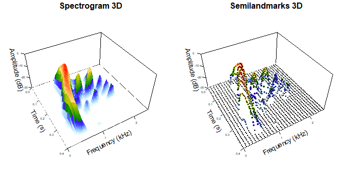
Figure 1: Graphical outputs using threeDspectro function from SoundShape package: (left) 3D spectrogram and (right) points (i.e. semilandmarks) sampled from 3D spectrogram data. cuvieri sample from SoundShape package.

# Traditional oscillogram and spectrogram
par(mfrow=c(1,2), mar=c(4,4,2,1)) # view side by side
seewave::oscillo(cuvieri.cut, title="Oscillogram")
seewave::spectro(cuvieri.cut, flim=c(0, 2.5), grid=FALSE, scale=FALSE, main="Spectrogram")

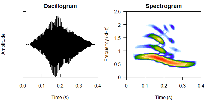
Figure 2: Graphical outputs using seewave package: (left) Oscillogram created with oscillo function and (right) 2D spectrogram created with spectro function. cuvieri sample from SoundShape package.

Installation

SoundShape package is currently available on R platform through the Comprehensive R Archive Network (CRAN) (https://CRAN.R-project.org/package=SoundShape). Alternatively, a development version is available from GitHub (https://github.com/p-rocha/SoundShape).

The package can be installed using one of the following codes:

# Official version from CRAN (recommended):
install.packages("SoundShape")

# Development version from GitHub:
install.packages("devtools")
devtools::install_github("p-rocha/SoundShape")

Citation

In case you wish to use and cite SoundShape package, use citation("SoundShape").

citation("SoundShape")
#> 
#> To cite package 'SoundShape' in publications use:
#> 
#>   Pedro Rocha (2021). SoundShape: Sound Waves Onto Morphometric Data. R
#>   package version 1.1.0. https://github.com/p-rocha/SoundShape
#> 
#> A BibTeX entry for LaTeX users is
#> 
#>   @Manual{,
#>     title = {SoundShape: Sound Waves Onto Morphometric Data},
#>     author = {Pedro Rocha},
#>     year = {2021},
#>     note = {R package version 1.1.0},
#>     url = {https://github.com/p-rocha/SoundShape},
#>   }

In addition, we recommend citing MacLeod et al. (2013) and Rocha & Romano (2021):

• MacLeod, N., Krieger, J., & Jones, K. E. (2013). Geometric morphometric approaches to acoustic signal analysis in mammalian biology. Hystrix, the Italian Journal of Mammalogy, 24(1), 110-125. doi: 10.4404/hystrix-24.1-6299.

• Rocha, P. & Romano, P. (2021) The shape of sound: A new R package that crosses the bridge between Bioacoustics and Geometric Morphometrics. Methods in Ecology and Evolution, 00, 1-7. doi: 10.1111/2041-210X.13580

Workflow using SoundShape package

1. Definition of homologous acoustic units

Since eigensound is centered around stereotyped acoustic units, the foremost step in sound shape study is the careful definition of units from which analysis will be conducted. However, even though several authors argue that acoustic traits constrained by anatomical structures (e.g. dominant frequency, pulse rate) are more conservative than those under the direct influence of behaviour (e.g. call duration, interval between calls), the criteria for homologous sound comparison may vary across different animal groups (see Rocha & Romano, 2021, for examples and more on homology between animal sounds). Therefore, we recommend a throughout literature review before the definition of acoustic units. Herein, we adopted a physiological definition of ‘note’, (McLister et al., 1995; Robillard et al., 2006), which led to an unambiguous selection of stereotyped calls from three frog species: Physalaemus centralis, P. cuvieri and P. kroyeri (centralis, cuvieri and kroyeri sample datas, respectively; Figs. 3 – 5).

# Samples of data from SoundShape package
data(cuvieri)
data(centralis)
data(kroyeri)

# Plot spectro from sample and highlight acoustic units

# centralis
seewave::spectro(centralis, flim = c(0, 4), wl=512, f=44100, ovlp=70, grid=FALSE)
graphics::abline(v=c(0.1, 0.8, 1.08, 1.78, 2.1, 2.8), lty=2)

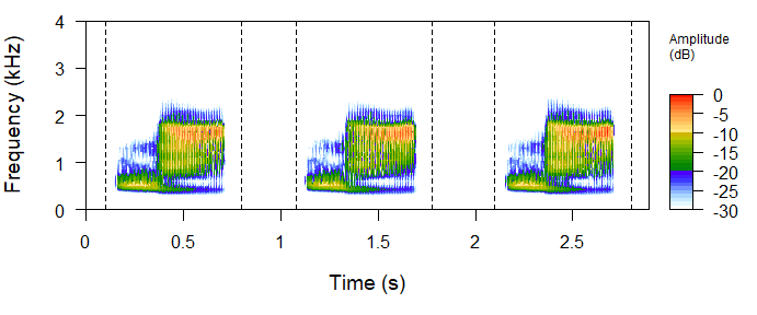
Figure 3: Spectrogram image of centralis sample (SoundShape package), containing a sequence of three stereotyped vocalizations, each representing a comparable acoustic unit.

# cuvieri
seewave::spectro(cuvieri, flim = c(0,4), wl=512, f=44100, ovlp=70, grid=FALSE)
graphics::abline(v=c(0.05, 0.45, 0.73, 1.13, 1.47, 1.87), lty=2)

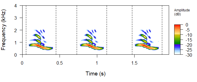
Figure 4: Spectrogram image of cuvieri sample (SoundShape package), containing a sequence of three stereotyped vocalizations, each representing a comparable acoustic unit.

# kroyeri
seewave::spectro(kroyeri, flim = c(0, 4), wl=512, f=44100, ovlp=70, grid=FALSE)
graphics::abline(v=c(0.16, 0.96, 1.55, 2.35, 2.9, 3.8), lty=2)

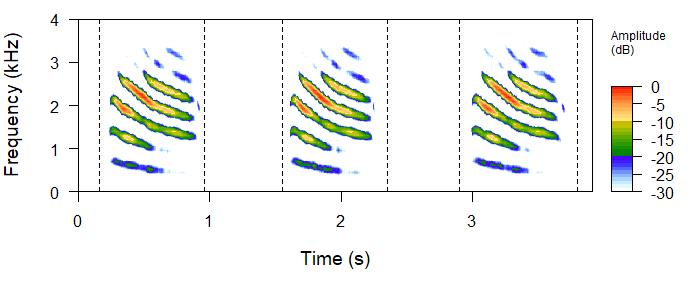
Figure 5: Spectrogram image of kroyeri sample (SoundShape package), containing a sequence of three stereotyped vocalizations, each representing a comparable acoustic unit.

2. Create folder to store acoustic units

The eigensound function (SoundShape package) focuses on the acquisition of point coordinates (i.e. semilandmarks) from multiple Waveform Audio File Format (WAV or WAVE; ".wav" file extensions), with each file representing a comparable acoustic unit (see section 1). These ".wav" files must be stored on the same folder somewhere in your computer, which can be created manually at your console and subsequently assigned as working directory in R.

Alternatively, one can create the folder at e.g. the current working directory using dir.create. Also create a subfolder to store the upcoming outputs from eigensound function, as the following:

# Create a folder to store ".wav" files
wav.at <- file.path(getwd(), "Workflow sample")
dir.create(wav.at)

# Create subfolder to store results
store.at <- file.path(getwd(), "Workflow sample/output")
dir.create(store.at)

3. Select and store acoustic units as separate ".wav" files

A reasonable number of comparable acoustic units should be selected from the sample and stored as new ".wav" files on a folder from your console (see section 2 for folder paths). Each file should represent a single unit selected from the original sound wave.

Since the slightest graphical change may incur in biased results (MacLeod et al., 2013; Rocha & Romano, 2021), acoustic units must be selected according to optimal signal to noise ratio (i.e. “clean” recording), and no overlapping frequencies from other individuals, species, or background noise. Editing and filtering of sound waves must be restricted to a bare minimum.

The selection can be performed on numerous softwares of acoustic analysis outside R platform (e.g.Audacity, Raven Pro), or using some functions from seewave and tuneR packages as exemplified below:

# Select acoustic units
cut.centralis <- seewave::cutw(centralis, f=44100, from=0, to=0.9, output = "Wave")
cut.cuvieri <- seewave::cutw(cuvieri, f=44100, from=0, to=0.9, output = "Wave")
cut.kroyeri <- seewave::cutw(kroyeri, f=44100, from=0.2, to=1.1, output = "Wave")

# Export ".wav" files containing acoustic units and store on previosly created folder
writeWave(cut.cuvieri, filename = file.path(wav.at, "cut.cuvieri.wav"), extensible = FALSE)
writeWave(cut.centralis, filename = file.path(wav.at, "cut.centralis.wav"), extensible = FALSE)
writeWave(cut.kroyeri, filename = file.path(wav.at, "cut.kroyeri.wav"), extensible = FALSE)

Alternatively, since SoundShape's version 1.3.0, the function raven.to.wave allows the creation of ".wav" files based on selections made using Raven Pro, which is commonplace in bioacoustical analysis. Each selection (i.e. line in table; see raven.list documentation) should represent an acoustic unit from the sample study:

###
## Using SoundShape examples:

# Export original sample ".wav" files
tuneR::writeWave(centralis, extensible = TRUE,
                filename = file.path(orig.wav, "centralis.wav"))
tuneR::writeWave(cuvieri, extensible = TRUE,
                filename = file.path(orig.wav, "cuvieri.wav"))
tuneR::writeWave(kroyeri, extensible = TRUE,
                filename = file.path(orig.wav, "kroyeri.wav"))

# Store Raven Pro selection tables at same folder from original ".wav" files
for(i in 1:length(raven.list)){
 write.table(raven.list[i], file=file.path(orig.wav, names(raven.list)[i]),
               quote=FALSE, sep="\t", row.names = FALSE,
               col.names = colnames(raven.list[[i]]))  } # end loop

# Verify if folder has both original ".wav" files and Raven's selections
dir(orig.wav)

###
## Start here when using your own recordings

# Export a ".wav" sample for each selection made in Raven Pro
raven.to.wave(orig.wav.folder = orig.wav, wav.samples = wav.at)

# Verify samples
dir(wav.at)

4. Three steps that avoid errors and biased results

The semilandmarks from eigensound function (SoundShape package) are automatically acquired, meaning that this approach does not add human errors from LM digitalization. Despite that, the eigensound protocol (MacLeod et al., 2013) requires some standardization to ".wav" files that would otherwise lead to errors or biased results (e.g. sounds overlapping the edges of a sound window; units far from the beginning of sound window; a low signal to noise ratio; Rocha & Romano, 2021).

In light of this, Rocha & Romano (2021) proposed the following steps that prevent errors and biased results, which are aided by the functions align.wave and eigensound (with analysis.type = "twoDshape"), both from SoundShape package.

4.1 Define dimensions for the sound window

First, define the sound window dimensions that encompass the whole sample of acoustic units. These dimensions are represented by the time (x-axis) and frequency (y-axis) limits for spectrogram images, which are respectively defined by the tlim and flim arguments in eigensound function.

Time limits should be based on the acoustic unit with the longest duration within the sample, whereas frequency limits should consider the unit with the largest frequency bandwidth. In the present sample study, for instance, the longest units are also the ones with broader frequency bandwidths (i.e.kroyeri sample; Fig. 6), with approximately 0.7 s duration and highest frequencies close to 3.5 kHz. Therefore, the sound window dimensions that encompass the whole sample can be defined with tlim = c(0, 0.8) and flim = c(0, 4).

This can be exemplified using spectro function from seewave package:

# Spectrogram plots using standardized sound window dimensions
par(mfrow=c(2,2), mar=c(4,4,2,2))
seewave::spectro(cut.centralis, flim=c(0, 4), tlim=c(0, 0.8), main="data(centralis)",
                 wl=512, f=44100, ovlp=70, grid=FALSE, scale=FALSE)
seewave::spectro(cut.cuvieri, flim=c(0, 4), tlim=c(0, 0.8), main="data(cuvieri)", 
                 wl=512, f=44100, ovlp=70, grid=FALSE, scale=FALSE)
seewave::spectro(cut.kroyeri, flim=c(0, 4), tlim=c(0, 0.8), main="data(kroyeri)", 
                 wl=512, f=44100, ovlp=70, grid=FALSE, scale=FALSE)

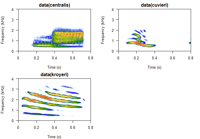
Figure 6: Spectrogram images with standardized sound window dimensions.

4.2 Alignment of acoustic units at the beginning of a sound window

The eigensound protocol also requires acoustic units to be placed at the beginning of a sound window before proceeding with the analysis. This ensures that variation in each semilandmark is due to energy shifts within the call, not to changes in their relative position in the sound window (MacLeod et al., 2013).

Although this arbitrary alignment could be performed on numerous software of acoustic analysis outside R platform (e.g.Audacity, Raven Pro), align.wave function (SoundShape package) provide an easy alternative to automatically align the units at the beginning of a sound window whilst also standardizing the durations of ".wav" files (see section 4.1), thus preventing errors when running eigensound function.

In order to verify the alignment, run eigensound with analysis.type = "twoDshape" and plot.exp = TRUE, which will create 2D spectrogram images and store them on the folder specified by store.at (see section 2 for folder paths), a helpful option for the verification of appropriate alignment and sound window dimensions.

Below is the code employed for the alignment of sound units and verification of sound window dimensions:

# Place sounds at the beginning of a sound window
align.wave(wav.at=wav.at, wav.to="Aligned", time.length = 0.8)

# Verify alignment using analysis.type = "twoDshape"
eigensound(analysis.type = "twoDshape", wav.at = file.path(wav.at, "Aligned"),
           store.at=store.at, plot.exp=TRUE, flim=c(0, 4), tlim=c(0, 0.8))

# Go to folder specified by store.at and check jpeg files created

If either the alignment, or the sound window dimensions, are not ideal (e.g. units far from the beginning of sound window; sounds overlapping the edges of sound window), run align.wave with different values of time.length and/or time.perc, then use eigensound to verify the updated spectrogram outputs (see Rocha & Romano, 2021 for details).

The ideal window dimensions and the alignment of units are often achieved after a few attempts. If this is troublesome, consider revisiting the relative amplitude (dBlevel) as the background noise could be interfering with align.wave (see section 4.3).

4.3 Set relative amplitude background

Next is the definition of a relative amplitude value (dBlevel) to be used as background in the 3D spectrogram (MacLeod et al., 2013). This is an iterative process that can be implemented by eigensound with analysis.type = "twoDshape" and plot.exp = TRUE, and should lead to spectrogram images with minimum influence from background noise (Rocha & Romano, 2021).

In the present study sample, the curve of relative amplitude was set at -25 dB (Fig. 5), which is expressed as an absolute value for dBlevel arguments in SoundShape functions (i.e.dBlevel = 25).

The code below was used to create the graphs from Fig. 7:

# 2D spectrogram with curves of relative amplitude at -25 dB
par(mfrow=c(1,2), mar=c(4,4,1,1))
s.kro <- seewave::spectro(cut.kroyeri, flim=c(0, 4), tlim = c(0, 0.8),  
                          grid=F, scale=F, f=44100, wl=512, ovlp=70, cont=TRUE, 
                          contlevels = seq(-25, -25, 1), collevels = seq(-40, 0, 0.1))
#> This took quite a lot of time to display this graphic, you may set 'fastdisp=TRUE' for a faster, but less accurate, display

# 3D spectrogram (with a lower dBlevel for illustrative purpuses)
threeDspectro(cut.kroyeri, dBlevel=40, flim=c(0, 4), tlim=c(0, 0.8), main="",
              colkey=list(plot=FALSE), cex.axis=0.4, cex.lab=0.8, resfac=2)

# Set background at -40 dB and remove -Inf values from spectrogram data 
for(i in 1:length(s.kro$amp)){if(s.kro$amp[i] == -Inf |s.kro$amp[i] <= -40)
{s.kro$amp[i] <- -40}}

# Add curve of relative amplitude
plot3D::contour3D(x=s.kro$time, y=s.kro$freq, colvar=t(s.kro$amp), z=-25,
                  plot=T, add=T, addbox=F, col="black", lwd=1.9, nlevels=2, dDepth=0.25)

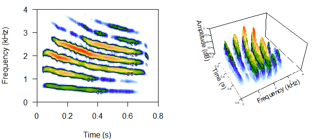
Figure 7: 2D and 3D spectrograms (left and right, respectively) with relative amplitude contours highlighted by black lines (dBlevel = 25). Spectrogram images from kroyeri sample.

5. Define sampling grid and run eigensound

After concluding the three steps that avoid errors and biased results (section 4), next is the definition of sampling grid dimensions that will be used for semilandmark acquisition (i.e. number of cells per side; x.length and y.length arguments, eigensound function; Fig. 8).

The number of cells per side will determine the amount of sLM acquired by eigensound. Therefore, the ideal grid should adequate the sound sample, while also representing a dimensionality reduction from spectrogram data (see Rocha & Romano, 2021). Herein, we opted for 70 cells on the time (x-axis, x.length = 70) and 47 cells on the frequency (y-axis, y.length = 47), which was experimentally defined with the aid of threeDspectro function, as exemplified below:

# Using threeDspectro to visualize sampling grid 
par(mfrow=c(1,2), mar=c(1,2,1,0)) 

# As "surface"
threeDspectro(cut.kroyeri, samp.grid=TRUE, x.length=70, y.length=47, plot.type="surface", 
              dBlevel=25, flim=c(0, 4), tlim=c(0, 0.8), f=44100, wl=512, ovlp=70, main="As 'surface'",
              colkey=list(plot=FALSE), cex.axis=0.4, cex.lab=0.8)

# As "points"
threeDspectro(cut.kroyeri, samp.grid=TRUE, x.length=70, y.length=47, plot.type="points", 
              dBlevel=25, flim=c(0, 4), tlim=c(0, 0.8), f=44100, wl=512, ovlp=70, main="As 'points'",
              colkey=list(plot=FALSE), cex.axis=0.4, cex.lab=0.8)

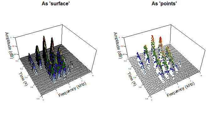
Figure 8: Spectrogram data as (left) simplified surface, and (right) colored semilandmarks acquired from the intersections of sampling grid (i.e.x.length=70 and y.length=47). Spectrogram images from kroyeri sample.

5.1 Run eigensound function

Once the three steps that avoid errors are concluded (section 4) and the sampling grid is defined (see above), it is now possible to acquire comparable semilandmark coordinates using eigensound function with analysis.type = "threeDshape".

Results can be simultaneosly assigned to an R object, and/or stored as the native file format of TPS series (Rohlf, 2015), a ".tps" file to be used by numerous software of geometric analysis of shape. Here, we focus on the analysis within R platform, so the results are assigned to the R object eig.sample, which is available as sample data from SoundShape.

Note:eig.sample comprises all vocalizations present in the samples of centralis, cuvieri and kroyeri, which led to three acoustic units per species; a total of nine ".wav" files stored in the same folder. Use help(eig.sample) and check Rocha & Romano (2021) for details.

In the following code, eigensound is run with a logarithmic scale on the time axis (i.e.log.scale = TRUE; see Rocha & Romano, 2021):

# Sample semilandmarks for each ".wav" file on a folder using a logarithmic sampling grid
# Export 3D graphs with semilandmarks as colored points for inspection
eig.sample <- eigensound(analysis.type="threeDshape", dBlevel=25, 
                         f=44100, wl=512, ovlp=70, flim=c(0, 4), tlim=c(0, 0.8),
                         x.length=70, y.length=47, log.scale=TRUE, plot.exp=TRUE, plot.type="points",
                         wav.at=file.path(wav.at, "Aligned"), store.at=store.at)

# Go to folder specified by store.at and check jpeg files created

6. Principal Components Analysis

After employing a sampling grid to acquire semilandmarks from sound waves (section 5), the eigensound protocol proceeds to a dimensionality reduction procedure that facilitate comparison of sound shape data. Herein, we opted for a Principal Components Analysis (PCA), which allow complex sound waves to be described and plotted onto major axes (PCs) encompassing the majority of variance within the sample (MacLeod et al., 2013; Rocha & Romano, 2021).

The PCA can be performed using prcomp function (stats package), as exemplified below:

# PCA using three-dimensional semilandmark coordinates embeeded in eig.sample
pca.eig.sample <- stats::prcomp(geomorph::two.d.array(eig.sample))

# View summary results
summary(pca.eig.sample)
#> Importance of components:
#>                             PC1      PC2      PC3      PC4      PC5     PC6
#> Standard deviation     125.0412 101.4575 39.39182 29.97205 17.11317 14.5307
#> Proportion of Variance   0.5407   0.3560  0.05367  0.03107  0.01013  0.0073
#> Cumulative Proportion    0.5407   0.8967  0.95041  0.98148  0.99161  0.9989
#>                            PC7     PC8       PC9
#> Standard deviation     4.95910 2.63948 5.762e-14
#> Proportion of Variance 0.00085 0.00024 0.000e+00
#> Cumulative Proportion  0.99976 1.00000 1.000e+00

Note: At this point, consider employing a stopping rule to select which PCs should be retained as nontrivial and interpretable, and which ones should be ignored (e.g. broken stick models, vegan package) (Jackson, 1993; see Rocha & Romano, 2021 for details).

6.1 Hypothetical sound shape configurations from semilandmark data

Before proceeding to the ordination of Principal Components (PCs), the eigensound protocol also includes hypothetical sound surfaces to be interpreted along with the ordination plots (MacLeod et al., 2013). These surfaces are calculated using hypo.surf function and should be interpreted along with the ordination plots, enhancing the comprehension of how sound shape changed along with each PCs

In SoundShape package, the hypothetical sound shapes can be created using hypo.surf function, which enables the calculation of either the mean shape configuration from the sample (i.e. consensus shape; Zelditch et al., 2012), or minimum and maximum deformations relative to PCs, as exemplified below:

# Create hypothetical sound surfaces using hypo.surf

# Mean shape configuration (consensus)
hypo.surf(eig.sample,  PC="mean", flim=c(0, 4), tlim=c(0, 0.8), x.length=70, y.length=47,
          cex.lab=0.7, cex.axis=0.5, cex.main=1)

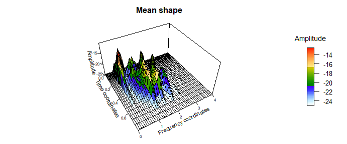
Figure 9: Hypothetical sound surface (acquired using hypo.surf function) representing mean shape configuration from eig.sample sample of data.

# Minimum and maximum deformations - Principal Component 1
hypo.surf(eig.sample, PC=1, flim=c(0, 4), tlim=c(0, 0.8), x.length=70, y.length=47,
          cex.lab=0.7, cex.axis=0.5, cex.main=1)

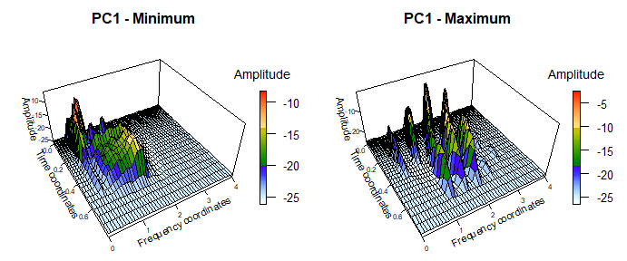
Figure 10: Hypothetical sound surfaces (acquired using hypo.surf function) representing minimum and maximum deformations relative to PC1 in the PCA featuring eig.sample sample of data.

# Minimum and maximum deformations - Principal Component 2
hypo.surf(eig.sample, PC=2, flim=c(0, 4), tlim=c(0, 0.8), x.length=70, y.length=47,
          cex.lab=0.7, cex.axis=0.5, cex.main=1)

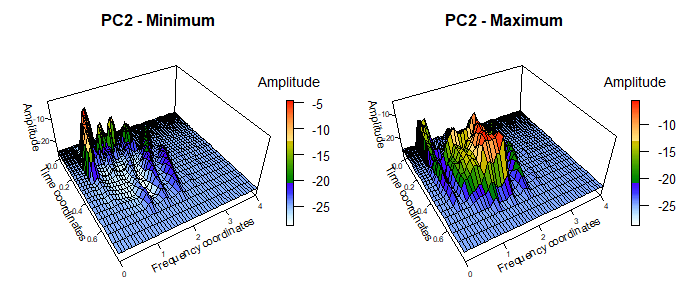
Figure 11: Hypothetical sound surfaces (acquired using hypo.surf function) representing minimum and maximum deformations relative to PC2 in the PCA featuring eig.sample sample of data.

6.2 Ordination plot with pca.plot function

Among the benefits of employing a PCA on multivariate data is the possibility to generate ordination plots encompassing the majority of variation embedded in the sample (Fig. 12). These plots simplify description and are widely employed in exploratory data analysis, specially when one is looking for potential groups within the sample (Zelditch et al. 2012).

The ordination plot is facilitated by pca.plot function (SoundShape package), which require the output of a PCA performed by prcomp function (stats package) and a vector with groups to be colored.

The code chunk below exemplifies how create an ordination plot using pca.plot:

# PCA using semilandmark coordinates
pca.eig.sample <- stats::prcomp(geomorph::two.d.array(eig.sample))

# Verify names of acoustic units from sample 
dimnames(eig.sample)[[3]]
#> [1] "cut.cent1" "cut.cent2" "cut.cent3" "cut.cuv1"  "cut.cuv2"  "cut.cuv3" 
#> [7] "cut.kro1"  "cut.kro2"  "cut.kro3"

# Based on those names, create factor to use as groups in subsequent ordination plot
sample.gr <- factor(c(rep("centralis", 3), rep("cuvieri", 3), rep("kroyeri", 3)))

# Ordination plot
pca.plot(pca.eig.sample, groups=sample.gr, conv.hulls=sample.gr, leg.pos="bottomright", cex=1.2)

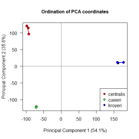
Figure 12: Ordination plot using eig.sample data acquired from the samples of centralis, cuvieri and kroyeri.

7. Interpreting the outputs of SoundShape

In order to fully comprehend how sound shape changes along the studied sample, the PCA outcome should be interpreted along with the visualization of hypothetical sound shapes (Figs. 9 – 11) and the ordination plot (Fig. 12).

The ordination plot (Fig. 12) represent 89.7% of the whole variance in our dataset, which yielded a clear structuring of units from different species. In addition, the hypothetical sound surfaces from the main axis of variation (i.e. mean shape and PCs) clearly represented the sound shapes of acoustic units employed in the study.

The higher positive values of PC1, for instance, corresponded to acoustic units with clear harmonic structure and broad frequency bandwidth (Fig. 10), a hypothetical sound shape remarkably similar to three-dimensional spectrograms from kroyeri sample. Not coincidently, the units from kroyeri scored high positive PC1 values. Lower and negative values of PC1, on the other hand, were less obvious, with a hypothetical shape that gather sonic information from cuvieri and centralis samples, both species with negative PC1 scores. A similar pattern is observed in PC2 axis (Fig. 11), with positive PC2 values referring to broad frequency bandwidth and no harmonic structure (i.e.centralis sample), and negative PC2 values representing short durations and clear harmonic structure (i.e.cuvieri sample).

References

Jackson, D. A. (1993). Stopping rules in Principal Components Analysis: A comparison of heuristical and statistical approaches. Ecology, 74(8), 2204-2214.

MacLeod, N., Krieger, J. & Jones, K. E. (2013). Geometric morphometric approaches to acoustic signal analysis in mammalian biology. Hystrix, the Italian Journal of Mammalogy, 24(1), 110-125. doi: 10.4404/hystrix-24.1-6299

McLister, J. D., Stevens, E. D., & Bogart, J. P. (1995). Comparative contractile dynamics of calling and locomotor muscles in three hylid frogs. The Journal of Experimental Biology, 198, 1527-1538.

Robillard, T., Hobel, G., & Gerhardt, H. C. (2006). Evolution of advertisement signals in North American hylid frogs: vocalizations as end-products of calling behavior. Cladistics, 22(6), 533-545. doi: 10.1111/j.1096-0031.2006.00118.x

Rocha, P. & Romano, P. (2021) The shape of sound: A new R package that crosses the bridge between Bioacoustics and Geometric Morphometrics. Methods in Ecology and Evolution, 00, 1-7. doi: 10.1111/2041-210X.13580

Rohlf, F.J. (2015) The tps series of software. Hystrix 26, 9-12.

Zelditch, M. L., Swiderski, D. L., Sheets, H. D., & Fink, W. L. (2012). Geometric morphometrics for biologists: A primer. Elsevier (Second Edition). Elsevier, San Diego.