Functions for Tidy Analysis and Generation of Random Data.

TidyDensity

The goal of {TidyDensity} is to make working with random numbers from different distributions easy. All tidy_ distribution functions provide the following components:

• [r_]
• [d_]
• [q_]
• [p_]

Installation

You can install the released version of {TidyDensity} from CRAN with:

install.packages("TidyDensity")

And the development version from GitHub with:

# install.packages("devtools")
devtools::install_github("spsanderson/TidyDensity")

Example

This is a basic example which shows you how to solve a common problem:

library(TidyDensity)
library(dplyr)
library(ggplot2)

tidy_normal()
#> # A tibble: 50 × 7
#>    sim_number     x       y    dx       dy     p       q
#>    <fct>      <int>   <dbl> <dbl>    <dbl> <dbl>   <dbl>
#>  1 1              1  0.991  -3.18 0.000487 0.839  0.991 
#>  2 1              2 -0.163  -3.05 0.00163  0.435 -0.163 
#>  3 1              3  2.19   -2.92 0.00454  0.986  2.19  
#>  4 1              4 -0.226  -2.78 0.0106   0.411 -0.226 
#>  5 1              5 -1.07   -2.65 0.0208   0.141 -1.07  
#>  6 1              6 -0.708  -2.52 0.0345   0.239 -0.708 
#>  7 1              7  0.343  -2.39 0.0488   0.634  0.343 
#>  8 1              8  0.264  -2.26 0.0600   0.604  0.264 
#>  9 1              9 -0.0531 -2.13 0.0667   0.479 -0.0531
#> 10 1             10  0.444  -2.00 0.0705   0.671  0.444 
#> # ℹ 40 more rows

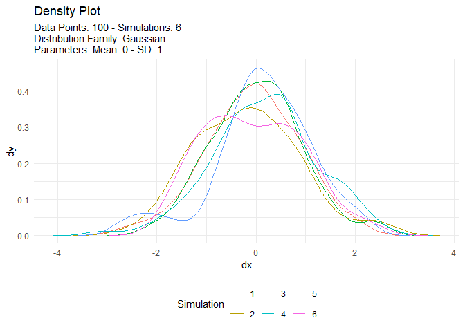
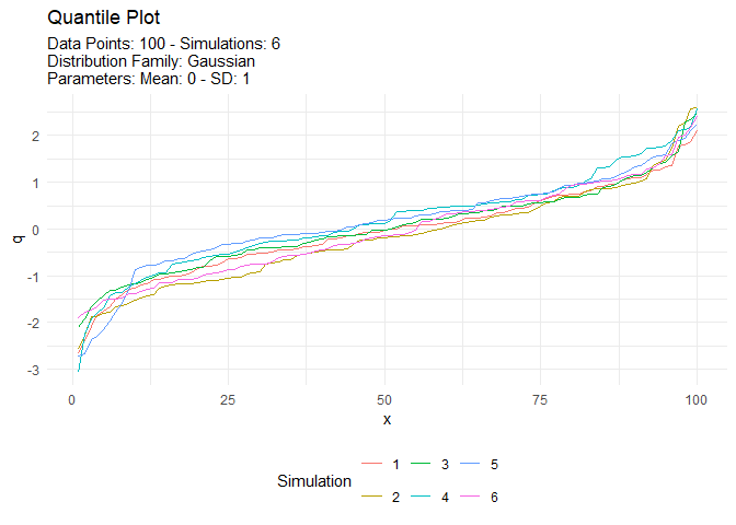
An example plot of the tidy_normal data.

tn <- tidy_normal(.n = 100, .num_sims = 6)

tidy_autoplot(tn, .plot_type = "density")

tidy_autoplot(tn, .plot_type = "quantile")

tidy_autoplot(tn, .plot_type = "probability")

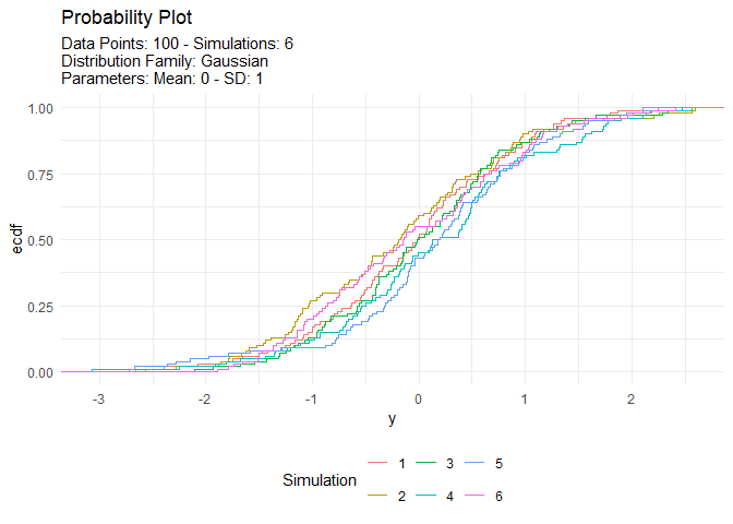
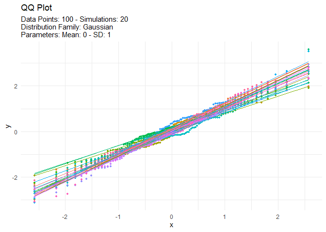
tidy_autoplot(tn, .plot_type = "qq")

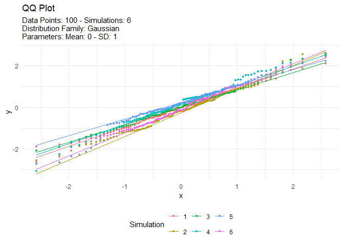
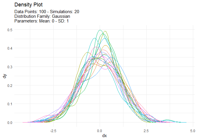
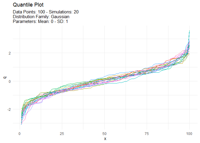
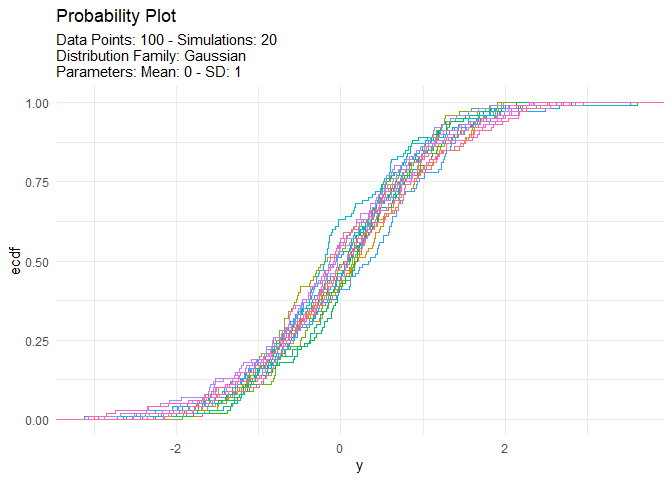
We can also take a look at the plots when the number of simulations is greater than nine. This will automatically turn off the legend as it will become too noisy.

tn <- tidy_normal(.n = 100, .num_sims = 20)

tidy_autoplot(tn, .plot_type = "density")

tidy_autoplot(tn, .plot_type = "quantile")

tidy_autoplot(tn, .plot_type = "probability")

tidy_autoplot(tn, .plot_type = "qq")