Toolkit for Investigation and Visualization of Young Anchovies.
Tivy
Toolkit for Investigation and Visualization of Young Anchovies
Tivy is an R package specialized in processing and analyzing fisheries data from Peru's anchovy (Engraulis ringens) fishery. It facilitates the handling of information from fishing trip logbooks, size records, hauls, and official announcements issued for preventive closures.
📋 Main Features
- 🐟 Data Processing: Automated processing of fishing hauls, trips, and length frequency data
- 🗺️ Spatial Analysis: Coordinate conversion, distance calculations, and fishing zone analysis
- 📊 Juvenile Analysis: Fish population structure analysis with length-weight relationships
- 📈 Visualization: Static (ggplot2) and interactive (leaflet) mapping capabilities
- 📋 Regulatory Integration: Processing of official fishing closure announcements
📦 Installation
You can install the development version of Tivy from GitHub:
# install.packages("devtools")
devtools::install_github("HansTtito/Tivy")
Install CRAN release:
install.packages("Tivy")
🚀 Usage Examples
Basic Loading and Processing
library(Tivy)

# Load and process logbook files
data_hauls <- process_hauls(
  data_hauls = calas_bitacora,
  correct_coordinates = TRUE,
  verbose = TRUE
)

data_fishing_trips <- process_fishing_trips(
  data_fishing_trips = faenas_bitacora,
  verbose = TRUE
)

hauls_length <- process_length(
  data_length = tallas_bitacora,
  verbose = TRUE
)
Data Integration
# Combination of length and fishing trip data
data_length_fishing_trips <- merge(
  x = data_fishing_trips,
  y = hauls_length,
  by = 'fishing_trip_code',
  all = TRUE
)

# Complete integration with haul data
data_total <- merge_length_fishing_trips_hauls(
  data_hauls = data_hauls,
  data_length_fishing_trips = data_length_fishing_trips
)

# Add derived variables (juveniles, distance to coast, etc.)
final_data <- add_variables(
  data = data_total,
  JuvLim = 12,  # Juvenile threshold in cm
  distance_type = "haversine",
  unit = "nm"
)
Juvenile Analysis
# Define length columns manually
length_cols <- as.character(seq(from = 8, to = 15, by = 0.5))

# Length-weight relationship parameters (for anchoveta)
a <- 0.0001
b <- 2.983

# Create catch column in tons
final_data$catch_t <- final_data$catch_ANCHOVETA / 1000

# Weight length frequencies according to catch
final_data_weighted <- apply_catch_weighting(
  data = final_data,
  length_cols = length_cols,
  catch_col = 'catch_t',
  a = a,  # Length-weight coefficient
  b = b   # Length-weight exponent
)

# Calculate juvenile proportion by group
juvenile_results <- summarize_juveniles_by_group(
  data = final_data_weighted,
  group_cols = c("dc_cat"),  # Distance category
  length_cols = paste0("weighted_", length_cols),
  juvenile_limit = 12,
  a = a,
  b = b
)

print(juvenile_results)
Visualization of Results
# Create date column for plotting
final_data_weighted$unique_date <- convert_to_date(final_data_weighted$start_date_haul)
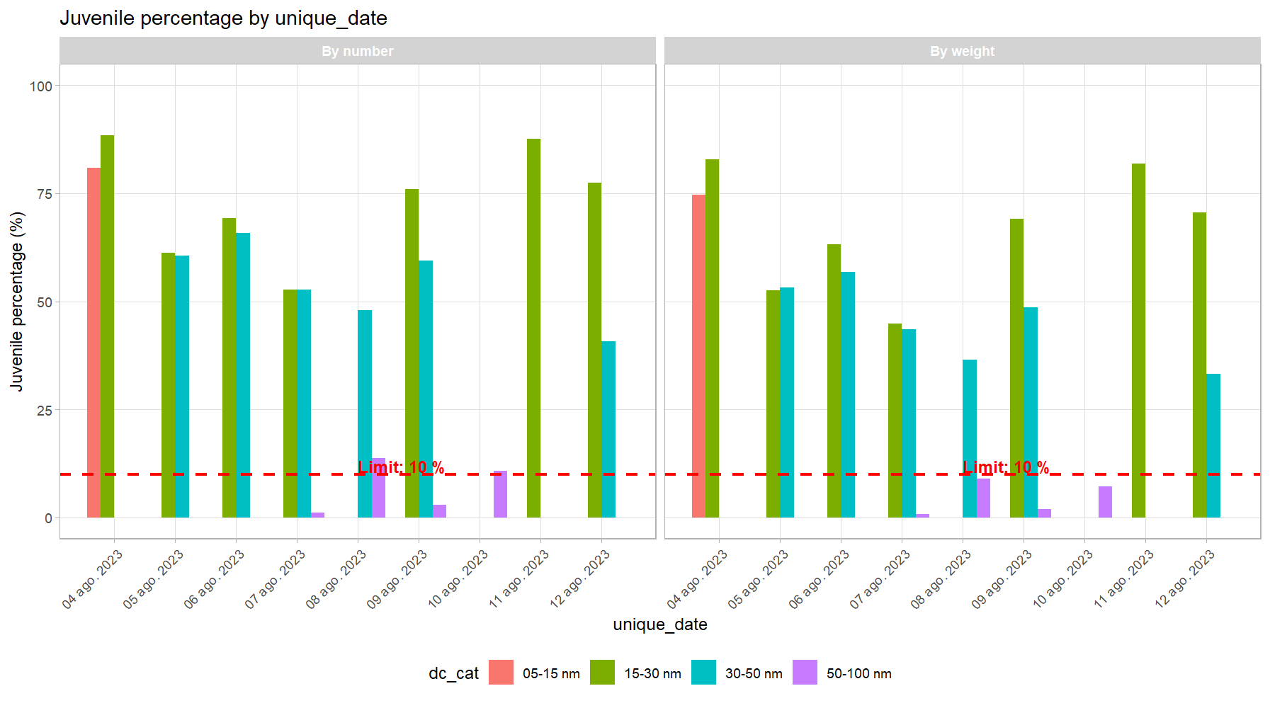
# Basic plot of juveniles by date
juvenile_plot <- plot_juvenile_analysis(
data = final_data_weighted,
x_var = "unique_date",
fill_var = "dc_cat",
length_cols = paste0("weighted_", length_cols),
a = a,
b = b,
reference_line = 10
)
print(juvenile_plot)
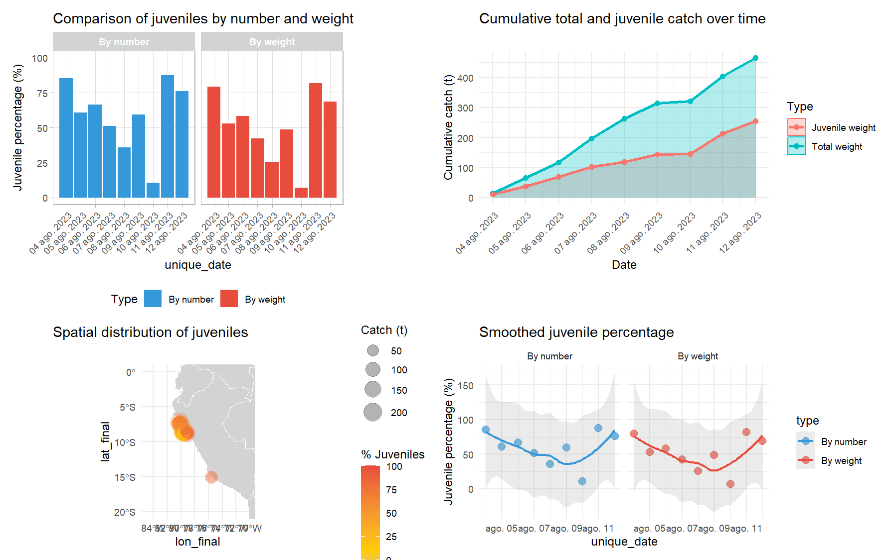
# Complete dashboard of juvenile analysis
dashboard <- create_fishery_dashboard(
  data = final_data_weighted,
  date_col = "unique_date",
  length_cols = paste0("weighted_", length_cols),
  a = a,
  b = b,
  latitude_col = "lat_initial",
  longitude_col = "lon_initial",
  catch_col = "catch_t",
  juvenile_col = "juv",
  date_breaks = "1 day"
)

# View individual dashboard components
dashboard$comparison      # Juvenile comparison
dashboard$trends         # Juvenile trends over time
dashboard$catch_trends   # Cumulative catch
dashboard$spatial_map    # Spatial distribution map
dashboard$dashboard      # Complete panel with all plots
Analysis of Official Announcements
# Fetch announcements from PRODUCE website
pdf_announcements <- fetch_fishing_announcements(
start_date = "01/03/2025",
end_date = "31/03/2025",
download = FALSE # Set TRUE to download PDF files
)
print(pdf_announcements)
# Extract information from PDF announcements
results <- extract_pdf_data(
pdf_sources = pdf_announcements$DownloadURL
)
# Format data for visualization
formatted_results <- format_extracted_data(
data = results,
convert_coordinates = TRUE
)
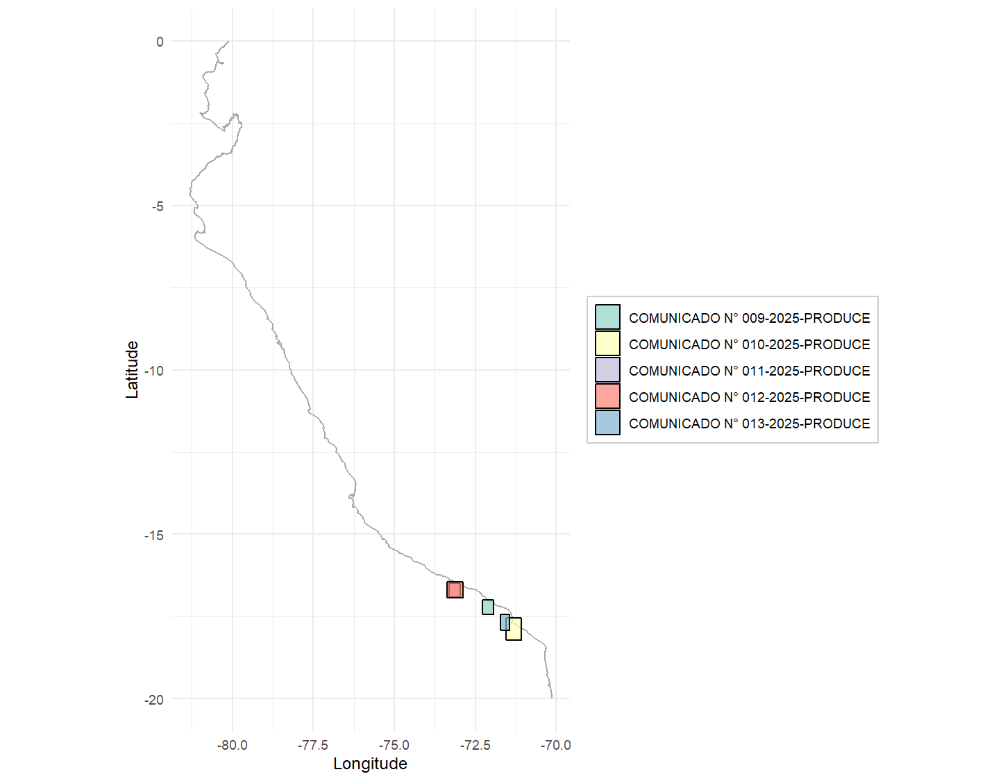
# Visualize closed areas with ggplot (static)
static_plot <- plot_fishing_zones(
data = formatted_results,
type = "static",
show_legend = TRUE,
title = "Fishing Closure Areas"
)
print(static_plot)
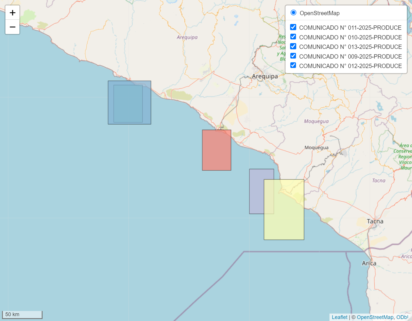
# Interactive visualization with leaflet
interactive_map <- plot_fishing_zones(
  data = formatted_results,
  type = "interactive",
  show_legend = TRUE,
  base_layers = TRUE,
  minimap = TRUE
)

interactive_map
📊 Recommended Workflow
- Load and process haul, fishing trip, and length data using
process_*()functions - Integrate datasets using
merge_length_fishing_trips_hauls() - Add derived variables with
add_variables()(distances, juveniles, etc.) - Prepare catch data by converting to appropriate units (tons)
- Apply catch weighting using
apply_catch_weighting()for biomass analysis - Analyze juvenile proportions by zones or seasons with
summarize_juveniles_by_group() - Create date columns for temporal analysis using
convert_to_date() - Visualize results through
plot_juvenile_analysis()orcreate_fishery_dashboard() - Integrate regulatory data using announcement processing functions
📄 Supported Data Structure
Tivy is designed to work with fishery data from Peru. The package includes built-in sample datasets:
calas_bitacora: Sample haul records with coordinates and catch datafaenas_bitacora: Sample fishing trip informationtallas_bitacora: Sample length frequency data- Official announcements: PDF documents with closure information from PRODUCE
🔧 Main Functions
| Category | Functions | Description |
|---|---|---|
| Data Processing | process_hauls(), process_fishing_trips(), process_length() | Data loading, cleaning, and standardization |
| Data Integration | merge_length_fishing_trips_hauls(), add_variables() | Data combination and variable enrichment |
| Spatial Analysis | dms_to_decimal(), coast_distance(), land_points() | Coordinate conversion and spatial calculations |
| Juvenile Analysis | apply_catch_weighting(), summarize_juveniles_by_group(), calculate_fish_weight() | Population structure and juvenile proportion analysis |
| Visualization | plot_juvenile_analysis(), plot_fishing_zones(), create_fishery_dashboard() | Static and interactive plotting |
| Announcements | fetch_fishing_announcements(), extract_pdf_data(), format_extracted_data() | Processing of official regulatory announcements |
| Utilities | convert_to_date(), find_columns_by_pattern(), validate_*_data() | Helper functions and data validation |
📚 Documentation
Comprehensive documentation is available through vignettes:
# Overview and quick start
vignette("introduction", package = "Tivy")

# Detailed data processing workflows
vignette("data-processing", package = "Tivy")

# Spatial analysis and mapping
vignette("spatial-analysis", package = "Tivy")

# Fish population analysis
vignette("fish-analysis", package = "Tivy")
Built-in Datasets
peru_coastline: Peruvian coastline coordinates for spatial analysisperu_coast_parallels: Parallel lines at different nautical mile distancescalas_bitacora: Sample haul datafaenas_bitacora: Sample trip datatallas_bitacora: Sample length data
Requirements
- R >= 4.0.0
- Required packages: dplyr, tidyr, lubridate, stringr, ggplot2, leaflet, RColorBrewer
- Suggested packages: future, patchwork, rnaturalearth (for enhanced functionality)
👩💻 Contributions
Contributions are welcome! Please consider:
- Opening an issue to discuss important changes
- Following the project's code style
- Including tests for new features
- Updating the corresponding documentation
📚 Citation
If you use Tivy in your research, please cite it as:
Ttito, H. (2025). Tivy: Tools for Fisheries Data Analysis in Peru.
R package version 0.1.1. https://github.com/HansTtito/Tivy
License
This project is licensed under the MIT License - see the LICENSE file for details.
Support
- 📖 Documentation: See package vignettes and function help pages
- 🐛 Bug reports: GitHub Issues
- 📧 Contact: [email protected]
Acknowledgments
- The R community for excellent packages that make this work possible
- Fisheries researchers and managers who provided feedback and requirements.