Respiratory Viral Infection Forecast Reporting.
ViroReportR
![]()
![]()
The goal of ViroReportR is to provide a toolbox to conveniently generate short-term forecasts (with accompanied diagnostics) for viral respiratory diseases.
Installation
ViroReportR depends on the latest version of the EpiEstim package (2.4). Thus, this version of the package must be installed from GitHub prior to installing the ViroReportR package using:
# install.packages("devtools")
install.packages('EpiEstim', repos = c('https://mrc-ide.r-universe.dev', 'https://cloud.r-project.org'))
You can then install the development version of ViroReportR from GitHub with:
devtools::install_github("BCCDC-PHSA/ViroReportR")
Quick Start
ViroReportR can be used to generate short-term forecasts with accompanied diagnostics in a few lines of code. We go through an example here where the EpiEstim backend is used to generate forecasts of Influenza-A, RSV and SARS-CoV-2.
library(ViroReportR)
library(tidyverse)
#> ── Attaching core tidyverse packages ──────────────────────── tidyverse 2.0.0 ──
#> ✔ dplyr     1.1.4     ✔ readr     2.1.5
#> ✔ forcats   1.0.0     ✔ stringr   1.6.0
#> ✔ ggplot2   4.0.0     ✔ tibble    3.2.1
#> ✔ lubridate 1.9.4     ✔ tidyr     1.3.1
#> ✔ purrr     1.0.2
#> ── Conflicts ────────────────────────────────────────── tidyverse_conflicts() ──
#> ✖ dplyr::filter() masks stats::filter()
#> ✖ dplyr::lag()    masks stats::lag()
#> ℹ Use the conflicted package (<http://conflicted.r-lib.org/>) to force all conflicts to become errors
library(ggplot2)
library(here)
#> here() starts at C:/Users/rebeca.falcao/ViroReportR
library(DT)
library(purrr)
library(kableExtra)
#>
#> Attaching package: 'kableExtra'
#>
#> The following object is masked from 'package:dplyr':
#>
#>     group_rows
We will use simulate_data to simulate date for Influenza A, RSV, and SARS-CoV-2, which is included with the ViroReportR package. We then pivot the simulated data to transform into a dataset with three columns: date, disease_type and confirm in accordance to format accepted by the model fitting functions.
diseases<-c("flu_a", "rsv", "sars_cov2")
data <- simulate_data(days=365, #days spanning simulation
                      peaks = c("flu_a"=90,"rsv"=110,"sars_cov2"=160), #peak day for each disease
                      amplitudes=c("flu_a"=50,"rsv"=40,"sars_cov2"=20), #amplitude of peak for each disease
                      scales = c("flu_a"=-0.004,"rsv"=-0.005,"sars_cov2"=-0.001), # spread of peak for each disease
                      time_offset = 0, #number of days to offset start of simulation
                      noise_sd = 5, #noise term
                      start_date = "2024-01-07" #starting day (Sunday)
                      )

data$date <- lubridate::ymd(data$date)

vri_data_list <- map2(rep(list(data), length(diseases)),
  diseases,~ get_aggregated_data(.x, "date", .y)) %>% set_names(diseases)

head(vri_data_list)
#> $flu_a
#> # A tibble: 366 × 2
#>    date       confirm
#>    <date>       <dbl>
#>  1 2024-01-07       0
#>  2 2024-01-08       8
#>  3 2024-01-09       0
#>  4 2024-01-10       5
#>  5 2024-01-11       0
#>  6 2024-01-12       8
#>  7 2024-01-13       9
#>  8 2024-01-14       0
#>  9 2024-01-15       4
#> 10 2024-01-16       0
#> # ℹ 356 more rows
#>
#> $rsv
#> # A tibble: 366 × 2
#>    date       confirm
#>    <date>       <dbl>
#>  1 2024-01-07       0
#>  2 2024-01-08       0
#>  3 2024-01-09       0
#>  4 2024-01-10       0
#>  5 2024-01-11       5
#>  6 2024-01-12       0
#>  7 2024-01-13       0
#>  8 2024-01-14       1
#>  9 2024-01-15       0
#> 10 2024-01-16       0
#> # ℹ 356 more rows
#>
#> $sars_cov2
#> # A tibble: 366 × 2
#>    date       confirm
#>    <date>       <dbl>
#>  1 2024-01-07       9
#>  2 2024-01-08       0
#>  3 2024-01-09       0
#>  4 2024-01-10       0
#>  5 2024-01-11       0
#>  6 2024-01-12       0
#>  7 2024-01-13       0
#>  8 2024-01-14       3
#>  9 2024-01-15       0
#> 10 2024-01-16       0
#> # ℹ 356 more rows
Model fitting and forecasting
The code below estimates the reproduction number using EpiEstim through the generate_forecast() function for each disease type via the purrr::map2() function. The generate_forecast() function prepares the data, estimates the reproduction number, and produces short-term forecasts of daily confirmed cases for an n_days forecast horizon. The other current choice for the forecasting algorithm is EpiFilter (WIP).
# parameters set-up
start_date <- min(data$date) + 13
n_days <- 14 # number of days ahead to forecast (n_days)
smooth <- FALSE # logical indicating whether smoothing should be applied in the forecast
forecasts_results <- tibble(
  vri_data_list,
  forecasts = map2(
    vri_data_list,
    diseases,
    ~ generate_forecast(
      data = .x,
      smooth_data = smooth,
      type = .y,
      n_days = n_days,
      start_date = start_date
    )
  )
)


names(forecasts_results$forecasts) <- diseases
names(forecasts_results$vri_data_list) <- diseases
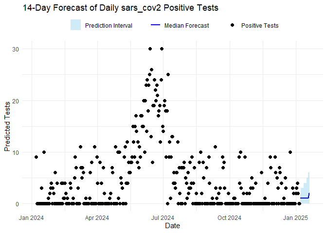
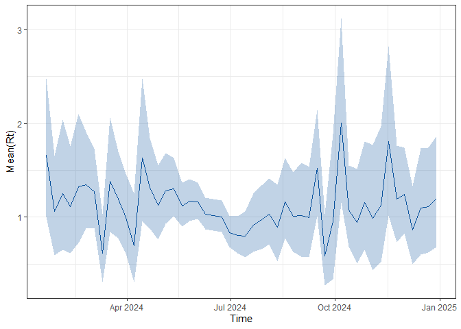
Plotting results
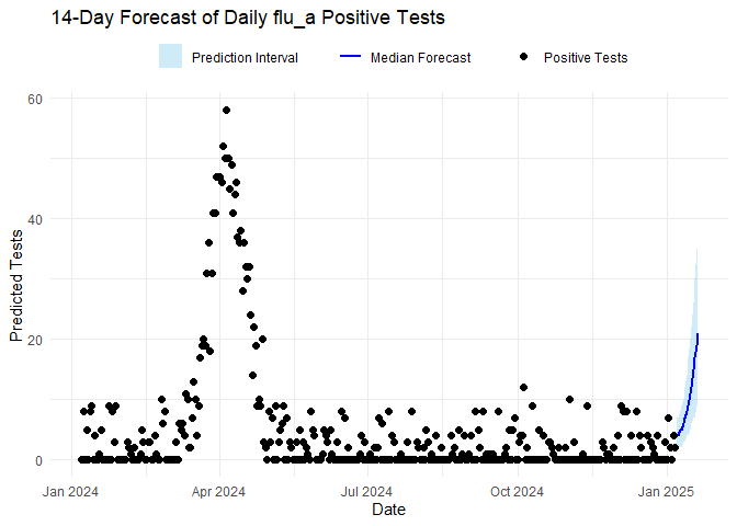
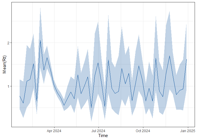
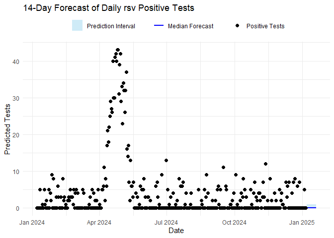
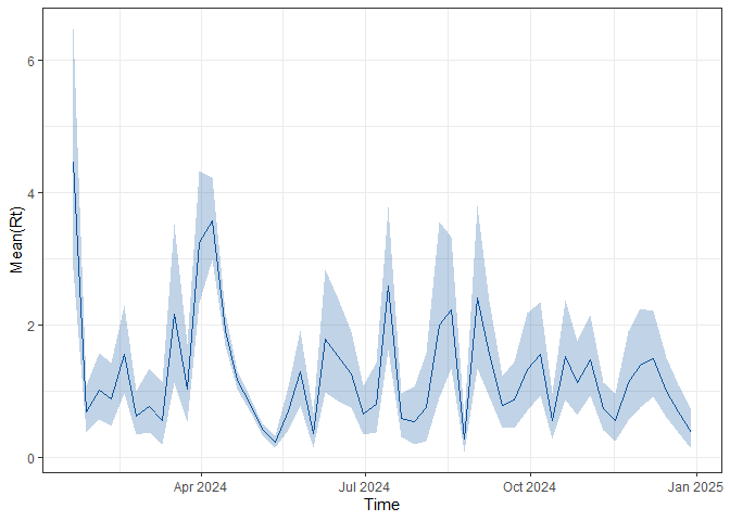
The code below plots the forecasts results and the estimated $R_t$ for each disease. To plot $R_t$, the code below uses plot_rt function included in the package.
for (vri in diseases) {
  forecast_plot <- ggplot() +
  geom_ribbon(
    data = forecasts_results$forecasts[[vri]][["forecast_res_quantiles"]],
    aes(x = date, ymin = p10, ymax = p90, fill = "Prediction Interval"),
    alpha = 0.4
  ) +
  geom_line(
    data = forecasts_results$forecasts[[vri]][["forecast_res_quantiles"]],
    aes(x = date, y = p50, color = "Median Forecast"),
    linewidth = 1
  ) +
  geom_point(
    data = forecasts_results$vri_data_list[[vri]],
    aes(x = date, y = confirm, shape = "Positive Tests"),
    size = 2,
    color = "black"
  )  +

  labs(
    title = paste0(n_days, "-Day Forecast of Daily ", vri, " Positive Tests"),
    x = "Date", y = "Predicted Tests",
    fill = "", color = "", shape = ""
  ) +
  scale_fill_manual(values = c("Prediction Interval" = "skyblue")) +
  scale_color_manual(values = c("Median Forecast" = "blue")) +
  scale_shape_manual(values = c("Positive Tests" = 16)) +
  theme_minimal() +
  theme(legend.position = "top", legend.direction = "horizontal")

  # create Rt plot
  rt_plot <- ViroReportR:::plot_rt(forecasts_results$forecasts[[vri]])
  print(forecast_plot)
  print(rt_plot)
}
Forecast report
Finally, the ViroReportR package can generate an automated report for the current season across all supported respiratory viruses (Influenza A, RSV, and SARS-CoV-2) using the generate_forecast_report() function. This function renders an HTML report summarizing model outputs and forecasts.
To use it, provide an input file (input_file) containing the required data with three columns—date, disease_type, and confirm—and specify an output directory (output_directory) where the report will be saved.
# rendering forecast report
df <- imap_dfr(vri_data_list, ~ .x %>% mutate(disease_type = .y))
input_file<-"simulated_data.csv"
write.csv(df, input_file, row.names = FALSE)
generate_forecast_report(
  input_data_dir =  input_file, # input filepath
  output_dir = output_directory, # output directory
  n_days = 14, # number of days to forecast
  validate_window_size = 7, # number of days between each validation window
  smooth = FALSE, # logical indicating whether smoothing should be applied in the forecast
)