Enhanced Implementation of Whittaker-Henderson Smoothing.

Revisiting Whittaker-Henderson Smoothing

What is Whittaker-Henderson smoothing ?

Whittaker-Henderson (WH) smoothing is a gradation method aimed at correcting the effect of sampling fluctuations on an observation vector. It is applied to evenly-spaced discrete observations. Initially proposed by Whittaker (1922) for constructing mortality tables and further developed by the works of Henderson (1924), it remains one of the most popular methods among actuaries for constructing experience tables in life insurance. Extending to two-dimensional tables, it can be used for studying various risks, including but not limited to: mortality, disability, long-term care, lapse, mortgage default, and unemployment.

How to use the package?

The WH package may easily be installed from CRAN by running the code install.packages("WH") in the $\mathsf{R}$ Console.

It features two main functions WH_1d and WH_2d corresponding to the one-dimensional and two-dimensional cases respectively. Two arguments are mandatory for those functions:

• The vector (or matrix in the two-dimension case) d corresponding to the number of observed events of interest by age (or by age and duration in the two-dimension case). d should have named elements (or rows and columns) for the model results to be extrapolated.

• The vector (or matrix in the two-dimension case) ec corresponding to the portfolio central exposure by age (or by age and duration in the two-dimension case) whose dimensions should match those of d. The contribution of each individual to the portfolio central exposure corresponds to the time the individual was actually observed with corresponding age (and duration in the two-dimension cas). It always ranges from 0 to 1 and is affected by individuals leaving the portfolio, no matter the cause, as well as censoring and truncating phenomena.

Additional arguments may be supplied, whose description is given in the documentation of the functions.

The package also embed two fictive agregated datasets to illustrate how to use it:

• portfolio_mortality contains the agregated number of deaths and associated central exposure by age for an annuity portfolio.

• portfolio_LTC contains the agregated number of deaths and associated central exposure by age and duration (in years) since the onset of LTC for the annuitant database of a long-term care portfolio.

# One-dimensional case
d <- portfolio_mort$d
ec <- portfolio_mort$ec

WH_1d_fit <- WH_1d(d, ec)
Using outer iteration / Brent method

# Two-dimensional case
keep_age <- which(rowSums(portfolio_LTC$ec) > 5e2)
keep_duration <- which(colSums(portfolio_LTC$ec) > 1e3)

d  <- portfolio_LTC$d[keep_age, keep_duration]
ec <- portfolio_LTC$ec[keep_age, keep_duration]

WH_2d_fit <- WH_2d(d, ec)
Using performance iteration / Nelder-Mead method

Functions WH_1d and WH_2d output objects of class "WH_1d" and "WH_2d" to which additional functions (including generic S3 methods) may be applied:

• The print function provides a glimpse of the fitted results

WH_1d_fit
An object fitted using the WH_1D function
Initial data contains 74 data points:
  Observation positions:  19  to  92 
Smoothing parameter selected: 13454 
Associated degrees of freedom: 7.5 
WH_2d_fit
An object fitted using the WH_2D function
Initial data contains 90 data points:
  First dimension:  75  to  89 
  Second dimension:  0  to  5 
Smoothing parameters selected: 301   2 
Associated degrees of freedom: 13 

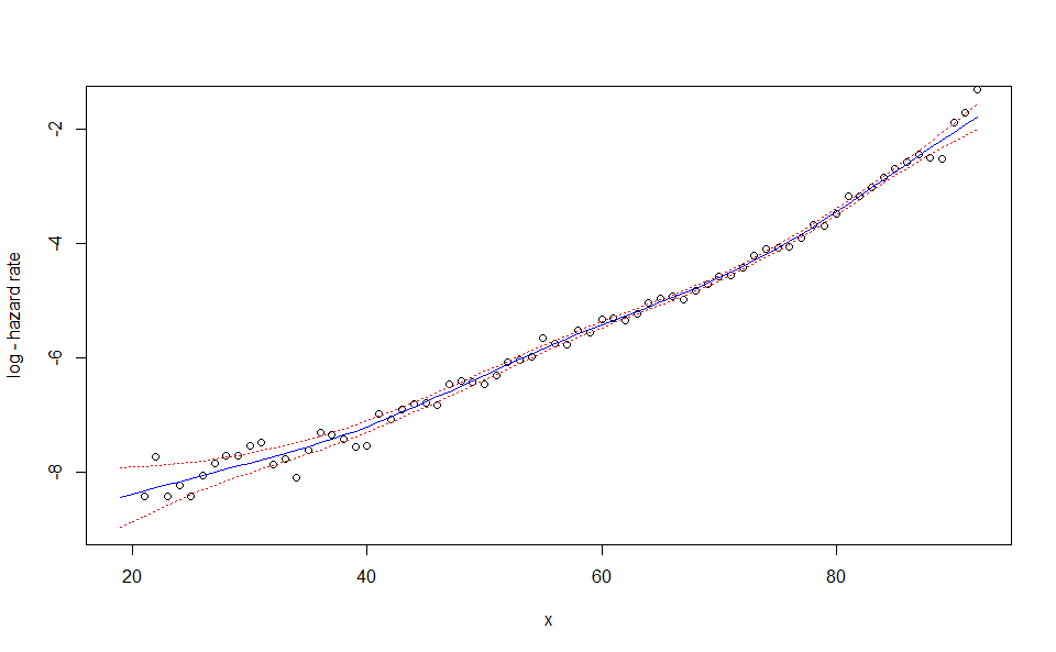
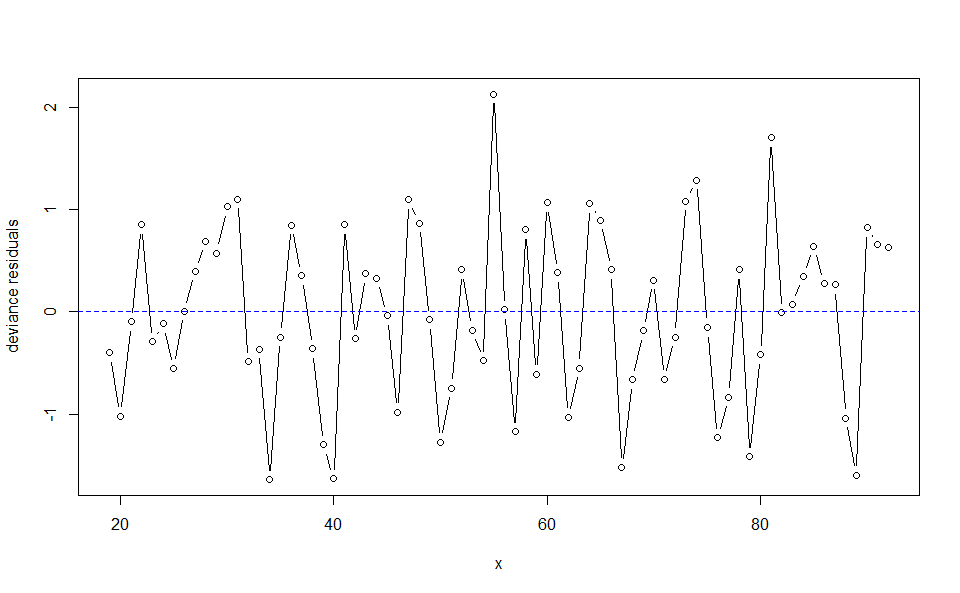
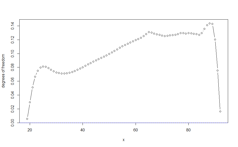
• The plot function generates rough plots of the model fit, the associated standard deviation, the model residuals or the associated degrees of freedom. See the plot.WH_1d and plot.WH_2d functions help for more details.

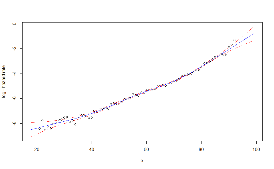
plot(WH_1d_fit)

plot(WH_1d_fit, "res")

plot(WH_1d_fit, "edf")

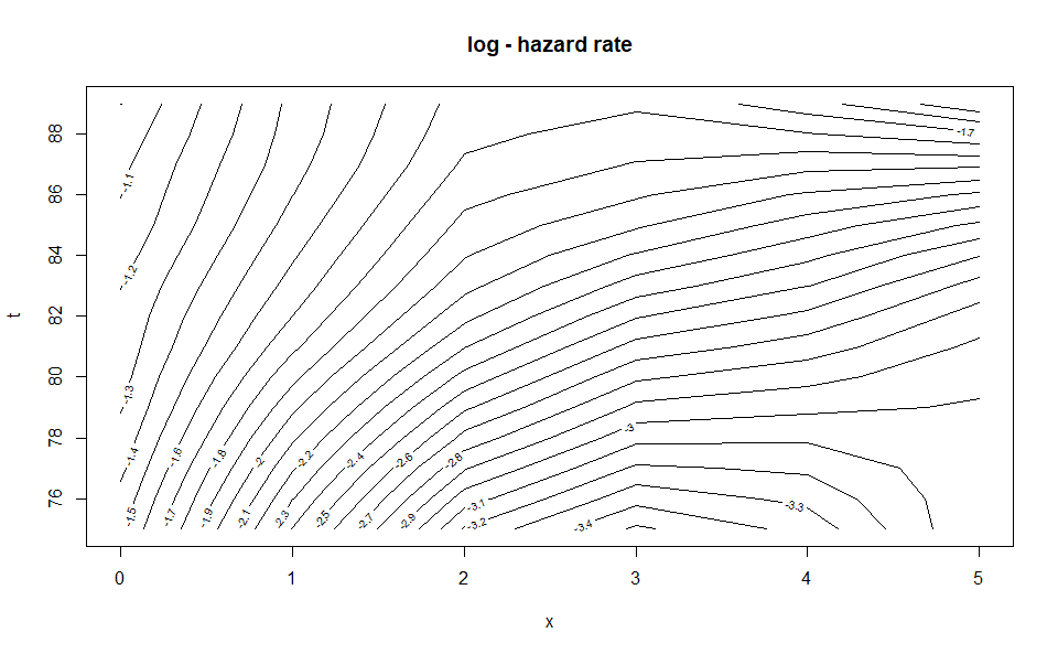
plot(WH_2d_fit)

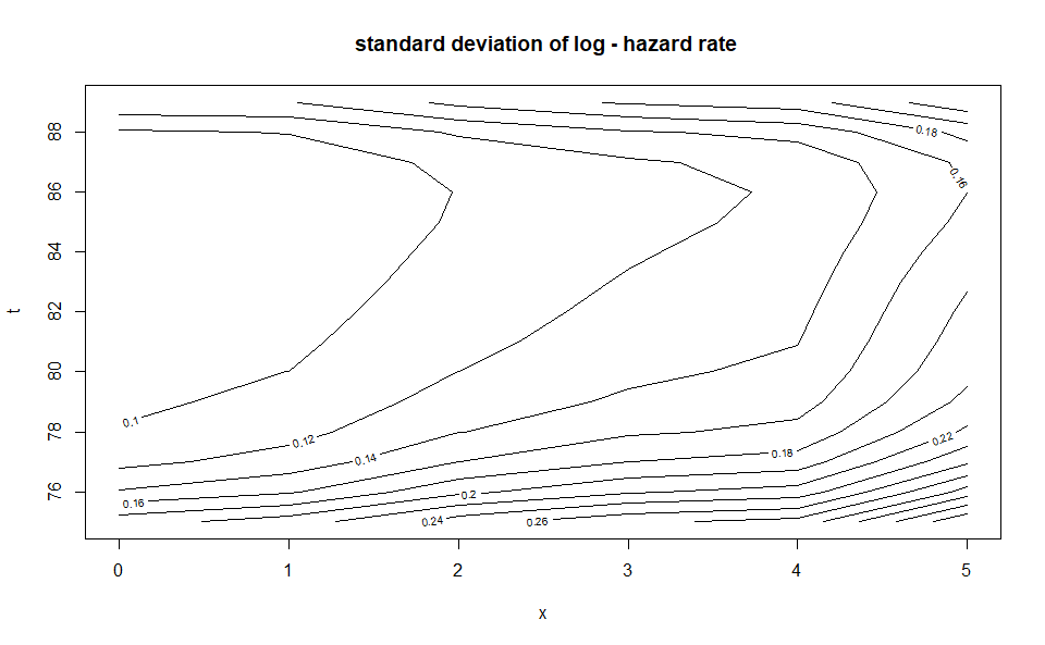
plot(WH_2d_fit, "std_y_hat")

• The predict function generates an extrapolation of the model. It requires a newdata argument, a named list with one or two elements corresponding to the positions of the new observations. In the two-dimension case constraints are used so that the predicted values matches the fitted values for the initial observations (see Carballo, Durban, and Lee 2021 to understand why this is required).

WH_1d_fit |> predict(newdata = 18:99) |> plot()

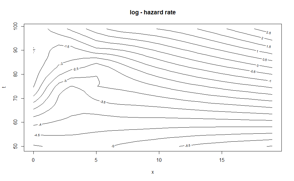
WH_2d_fit |> predict(newdata = list(age = 50:99,
                                    duration = 0:19)) |> plot()

• Finally the output_to_df function converts an "WH_1d" or "WH_2d" object into a data.frame. Information about the fit is discarded in the process. This function may be useful to produce better visualizations from the data, for example using the ggplot2 package.

WH_1d_df <- WH_1d_fit |> output_to_df()
WH_2d_df <- WH_2d_fit |> output_to_df()

Further WH smoothing theory

See the package vignette or the upcoming paper available here

References

Carballo, Alba, Maria Durban, and Dae-Jin Lee. 2021. “Out-of-Sample Prediction in Multidimensional p-Spline Models.” Mathematics 9 (15): 1761.
Henderson, Robert. 1924. “A New Method of Graduation.” Transactions of the Actuarial Society of America 25: 29–40.
Whittaker, Edmund T. 1922. “On a New Method of Graduation.” Proceedings of the Edinburgh Mathematical Society 41: 63–75.