Alternating Direction Method of Multipliers to Solve Dense Dubmatrix Problem.

admmDensenstSubmatrix

Introduction

This is the R-package accompanying the paper Convex optimization for the densest subgraph and densest submatrix problems.

See also Matlab-code

The problem of identifying a dense submatrix is a fundamental problem in the analysis of matrix structure and complex networks. This package provides tools for identifying the densest submatrix of the fixed size in a given graph/matrix using first-order optimization methods.

See the tutorials below to get started.

Installation

#Install the development version from GitHub:
# install.packages("remotes")
remotes::install_github("pbombina/admmDensenstSubmatrix")

To also build the vignettes use:

#install.packages("remotes")
remotes::install_github("pbombina/admmDensenstSubmatrix", dependencies = TRUE,
                         build_vignettes = TRUE)

Usage

This section gives a brief overview of the different functions included in this package. For more details use help('function') or doc('function').

R-package contains the functions:

• plantedsubmatrix.R generates binary matrix sampled from dense submatrix of particular size
• densub.R ADMM algorithm for our relaxation of the densest subgraph and submatrix problems
• mat_shrink.R soft-threholding operator applied to vector of singular values (used in X-update step of densub.R)

Examples

We test this package on two different types of data: first, using random matrices sampled from the planted dense m x n submtarix model and, second, real-world collaboration and communication networks.

Random matrices

We first generate a random matrix with noise obscuring the planted submatrix using the function plantedsubmatrix. and then call the function densub to recover the planted submatrix.

# Initialize problem size and densities
# You can play around with these parameters
M <- 100 #number of rows of sampled matrix
N <- 200 #number of columns of sampled matrix
m <- 50 #number of rows of dense submatrix
n <- 40 #number of columns of dense submatrix
p <- 0.25 # noise density
q <- 0.85 #in-group density

#Make binary matrix with mn-submatrix
random<-plantedsubmatrix(M = M, N = N,m = m,n = n,p = p,q = q)

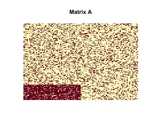
After generating the structure random containing the random matrix with desired planted structure, we can visually represent the matrix and planted submatrix as two-tone images, where dark pixels correspond to nonzero entries, and light pixels correspond to zero entries, using the following commands.

# Plot sampled G and matrix representations.
image(random$sampled_matrix, useRaster = TRUE, axes = FALSE, main = "Matrix A")
image(random$dense_submatrix, useRaster = TRUE, axes = FALSE, main = "Matrix X0")
image(random$disagreements, useRaster = TRUE, axes = FALSE, main = "Matrix Y0")

Tne vizualization of the randomly generated matrix helps us to understand its structure. It is clear that contains a dense block (in the bottom left corner).

We can remove all noise and isolate an image of a rank-one matrix with nonzero entries.

Then we vizualize matrix to see the number of disagreements between original matrix and .

We call the ADMM solver and visualize the output using the following commands.

#Call ADMM solver
admm <- densub(G = random$sampled_matrix, m = m, n = n, tau = 0.35, gamma = 6/(sqrt(m*n)*(q-p)), opt_tol = 1.0e-4,maxiter = 500, quiet = TRUE)


#Plot results
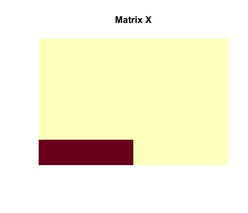
image(admm$X, useRaster = TRUE, axes = FALSE, main = "Matrix X")
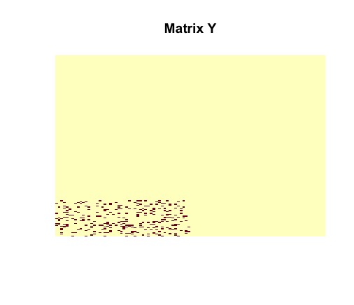
image(admm$Y, useRaster = TRUE, axes = FALSE, main = "Matrix Y")

The ADMM solver returns the optimal solutions and . It must be noted that matrices and are identical to the actual structures of and . The planted submatrix is recovered.

Collaboration Network

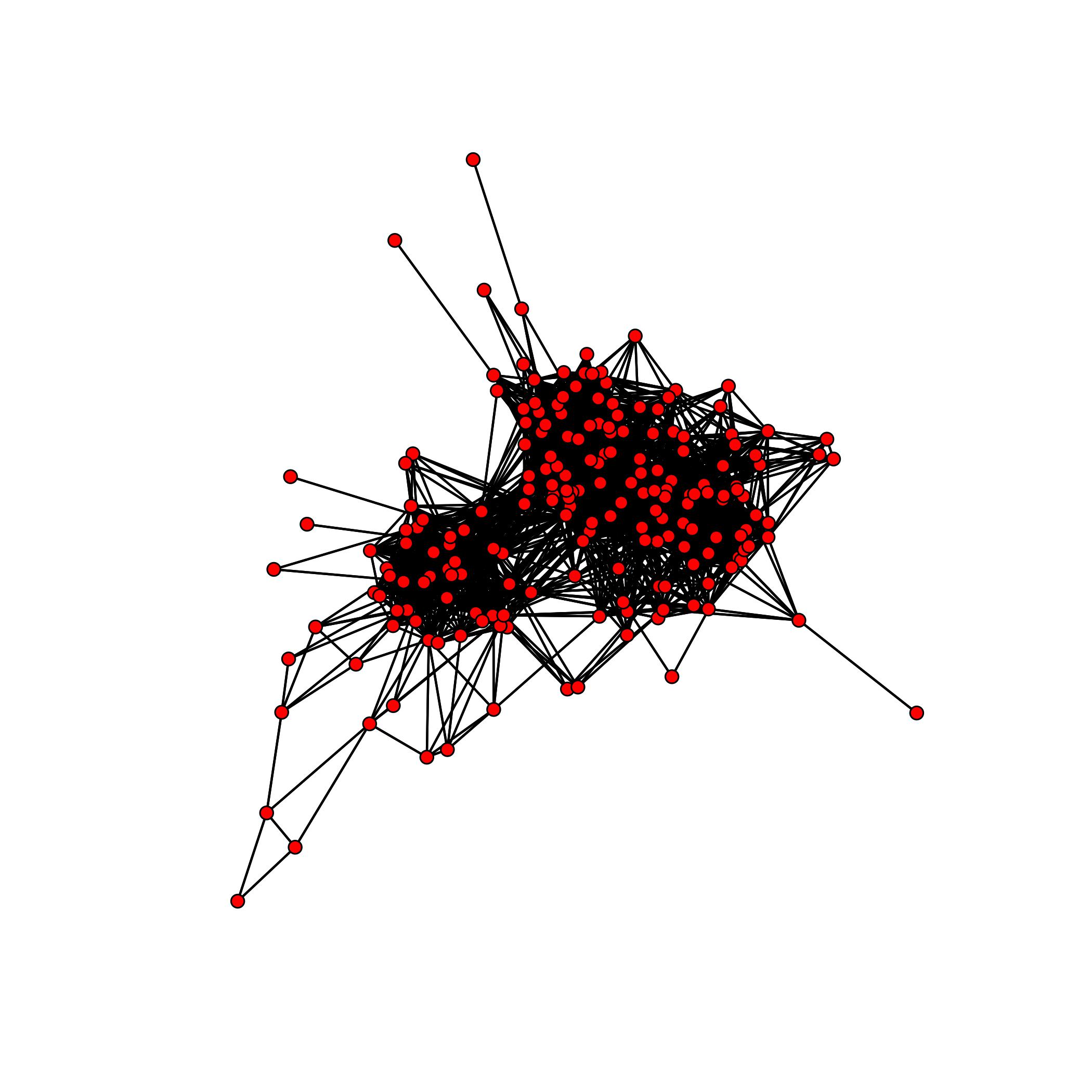
The following is a simple example on how one could use the package to analyze the collaboration network found in the JAZZ dataset. It is known that this network contains a cluster of 100 musicians which performed together.

We have already prepared dataset to work with. More details can be found in the provided file JAZZ_IN_R.R ( in vignettes folder).

#Load dataset
load(file = "JAZZ.RData") 

#Initialize problem size and densities
G <- new #define matrix G equivalent to JAZZ dataset 
m <- 100 #clique size or the number of rows of the dense submatrix 
n <- 100 #clique size of the number of columns of the dense sumbatrix
tau <- 0.85 #regularization parameter
opt_tol <- 1.0e-2 #optimal tolerance
maxiter <- 2000 #number of iterations
gamma <- 8/n #regularization parameter

#call ADMM solver
admm <- densub(G = G, m = m, n = n, tau = tau, gamma = gamma, opt_tol = opt_tol, maxiter=maxiter, quiet = TRUE) 

# Planted solution X0
X0 <- matrix(0L, nrow = 198, ncol = 198) #construct rank-one matrix X0
X0[1:100,1:100] <- matrix(1L, nrow = 100, ncol = 100)#define dense block

# Planted solution Y0
Y0 <- matrix(0L, nrow = 198, ncol = 198) #construct matrix for counting disagreements between G and X0
Y0[1:100,1:100] < matrix(1L,nrow = 100,ncol = 1000)-G[1:100,1:100]  

#Check primal and dual residuals
C <- admm$X-X0 
a <- norm(C, "F") #Frobenius norm of matrix C 
b <- norm(X0,"F") #Frobenius norm of matrix X0
recovery <- matrix(0L,nrow = 1, ncol = 1)#create recovery condition matrix

if (a/b^2<opt_tol){ #Recovery condition 
recovery = recovery+1
} else {
  recovery = 0 
  }

Our algorithm converges to the dense submatrix representing the community of 100 musicians after 50 iterations.

How to contribute

• Fork, clone, edit, commit, push, create pull request
• Use RStudio

Reporting bugs and other issues

If you encounter a clear bug, please file a minimal reproducible example on github.