Experimental Evaluation of Algorithm-Assisted Human Decision-Making.
aihuman
![]()
Overview
aihuman provides statistical methods for analyzing experimental evaluation of the causal impacts of algorithmic recommendations on human decisions developed by Imai, Jiang, Greiner, Halen, and Shin (2023).
The data used for this paper, and made available here, are interim, based on only half of the observations in the study and (for those observations) only half of the study follow-up period. We use them only to illustrate methods, not to draw substantive conclusions.
Installation
You can install the development version of aihuman from GitHub with:
# install.packages("devtools")
devtools::install_github("sooahnshin/aihuman", dependencies = TRUE, build_vignettes = TRUE)
If you have trouble with compilation on macOS, you may want to check this link.
Usage 1: Evaluation Based on Principal Stratification
The package provides main functions for the methods proposed by Imai, Jiang, Greiner, Halen, and Shin (2023) based on principal stratification.
| Category | Function | Type | Main Input | Output | Paper | Notes |
|---|---|---|---|---|---|---|
| descriptive | PlotStackedBar() | vis. | e.g., data(psa_synth) | ggplot | Fig 1 | dist. of $D_i$ |
| descriptive | CalDIMsubgroup() | est. | e.g., data(synth) | dataframe | Sec 2.4 | diff-in-means |
| descriptive | PlotDIMdecisions() | vis. | output of CalDIMsubgroup() | ggplot | Fig 2 (left) | |
| descriptive | PlotDIMoutcomes() | vis. | output of CalDIMsubgroup() for each outcome | ggplot | Fig 2 (right) | |
| main | AiEvalmcmc() | est.(c/h) | e.g., data(synth) | mcmc | Sec S5 | |
| main | CalAPCE() | est.(c/h) | output of PSAmcmc() | list | Sec 3.4 | |
| main | APCEsummary() | est. | output of CalAPCE() | dataframe | Sec 3.4 | APCE |
| main | PlotAPCE() | vis. | output of APCEsummary() | ggplot | Fig 4 | |
| strata | CalPS() | est. | $P.R.mcmc of CalAPCE() | dataframe | Eq 6 | $e_r$ |
| strata | PlotPS() | vis. | output of CalPS() | ggplot | Fig 3 | |
| fairness | CalFairness() | est. | output of CalAPCE() | dataframe | Sec 3.6 | $\Delta_r(z)$ |
| fairness | PlotFairness() | est. | output of CalFairness() | ggplot | Fig 5 | |
| optimal | CalOptimalDecision() | est. | output of AiEvalmcmc() | dataframe | Sec 3.7 | $\delta^\ast(\mathbf{x})$ |
| optimal | PlotOptimalDecision() | vis. | output of CalOptimalDecision() | ggplot | Fig 6 | |
| comparison | PlotUtilityDiff() | vis. | output of CalOptimalDecision() | ggplot | Fig 7 | $g_d(\mathbf{x})$ |
| comparison | PlotUtilityDiffCI() | vis. | output of CalOptimalDecision() | ggplot | Fig S17 | |
| crt | SpilloverCRT() | est. | court event hearing date, $D_i$, $Z_i$ | daraframe | Sec S3.1 | |
| crt | PlotSpilloverCRT() | vis. | output of SpilloverCRT() | ggplot | Fig S8 | |
| crt power | SpilloverCRTpower() | est. | court event hearing date, $D_i$, $Z_i$ | dataframe | Sec S3.2 | |
| crt power | PlotSpilloverCRTpower() | vis. | output of SpilloverCRTpower() | ggplot | Fig S9 | |
| frequentist | CalAPCEipw() | est. | e.g., data(synth) | dataframe | Sec S7 | |
| frequentist | BootstrapAPCEipw() | est. | e.g., data(synth) | dataframe | ||
| frequentist | APCEsummaryipw() | est. | outputs of CalAPCEipw() and BootstrapAPCEipw() | dataframe | ||
| frequentist (RE) | CalAPCEipwRE() | est. | e.g., data(synth) | dataframe | ||
| frequentist (RE) | BootstrapAPCEipwRE() | est. | e.g., data(synth) | dataframe |
vis. = visualization; est. = estimation; c/h = computation-heavy. You may use CalAPCEparallel() instead of CalAPCE() throughout the analysis.
For more details, see the aihuman package vignette, vignette("aihuman", package = "aihuman").
Example
library(aihuman)
## Using synthetic data with small run
data(synth)
sample_mcmc <- AiEvalmcmc(data = synth, n.mcmc = 10)
#> 10/10 done.
subgroup_synth <- list(1:nrow(synth),
which(synth$Sex == 0),
which(synth$Sex == 1),
which(synth$Sex == 1 & synth$White == 0),
which(synth$Sex == 1 & synth$White == 1))
sample_apce <- CalAPCE(data = synth,
mcmc.re = sample_mcmc,
subgroup = subgroup_synth)
# You can also use the parallelized version: check CalAPCEparallel()
sample_apce_summary <- APCEsummary(sample_apce[["APCE.mcmc"]])
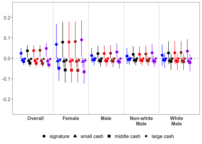
PlotAPCE(sample_apce_summary,
y.max = 0.25,
decision.labels = c("signature", "small cash", "medium cash", "large cash"),
shape.values = c(16, 17, 15, 18),
col.values = c("blue", "black", "red", "brown", "purple"),
label = FALSE)
Usage 2: Evaluation With Minimal Assumptions
The package provides main functions for the methods proposed by Ben-Michael, Greiner, Huang, Imai, Jiang, and Shin (2024) based on a minimal set of assumptions.
| Category | Function | Type | Output | Figure # |
|---|---|---|---|---|
| Human+AI v. Human | compute_stats_aipw() | est. | dataframe | |
| Human+AI v. Human | plot_diff_human_aipw() | vis. | ggplot | Fig 1 |
| AI v. Human | compute_bounds_aipw() | est. | dataframe | |
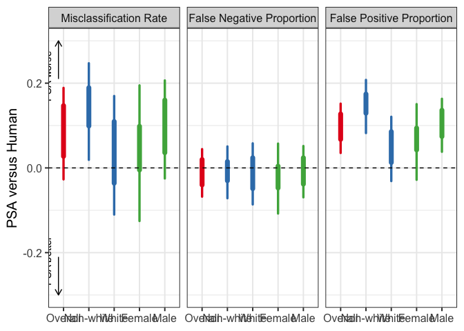
| AI v. Human | plot_diff_ai_aipw() | vis. | ggplot | Fig 2, 5, S4 |
| Preference | plot_preference() | vis. | ggplot | Fig 3, S5 |
| Agreement | table_agreement() | est | ggplot | |
| Agreement | plot_agreement() | vis. | ggplot | Fig S1 |
| Overrides | plot_diff_subgroup() | vis. | ggplot | Fig S2, S3 |
| Policy learning | See the vignette | vis. | ggplot | Fig 4 |
For more details, see the ablity vignette, vignette("ability", package = "aihuman").
Example
library(ggplot2)
## set default ggplot theme
theme_set(theme_bw(base_size = 15) + theme(plot.title = element_text(hjust = 0.5)))

## Human+AI v. Human
plot_diff_human_aipw(
  Y = NCAdata$Y,
  D = ifelse(NCAdata$D == 0, 0, 1),
  Z = NCAdata$Z,
  nuis_funcs = nuis_func,
  true.pscore = rep(0.5, nrow(NCAdata)),
  l01 = 1,
  subgroup1 = ifelse(NCAdata$White == 1, "White", "Non-white"),
  subgroup2 = ifelse(NCAdata$Sex == 1, "Male", "Female"),
  label.subgroup1 = "Race",
  label.subgroup2 = "Gender",
  x.order = c("Overall", "Non-white", "White", "Female", "Male"),
  p.title = NULL, p.lb = -0.3, p.ub = 0.3
)
## AI v. Human
plot_diff_ai_aipw(
  Y = NCAdata$Y,
  D = ifelse(NCAdata$D == 0, 0, 1),
  Z = NCAdata$Z,
  A = PSAdata$DMF,
  z_compare = 0,
  nuis_funcs = nuis_func,
  nuis_funcs_ai = nuis_func_ai,
  true.pscore = rep(0.5, nrow(NCAdata)),
  l01 = 1,
  subgroup1 = ifelse(NCAdata$White == 1, "White", "Non-white"),
  subgroup2 = ifelse(NCAdata$Sex == 1, "Male", "Female"),
  label.subgroup1 = "Race",
  label.subgroup2 = "Gender",
  x.order = c("Overall", "Non-white", "White", "Female", "Male"),
  zero.line = TRUE, arrows = TRUE, y.min = -Inf,
  p.title = NULL, p.lb = -0.3, p.ub = 0.3
)