Computes Bias-Adjusted Treatment Effect.

Bias-Adjusted Treatment Effect (bate)

Four Regressions

The goal of the bate package is to present some functions to compute quantiles of the empirical distribution of the bias-adjusted treatment effect (BATE) in a linear econometric model with omitted variables. To analyze such models, a researcher should consider four regression models: (a) a short regression model where the outcome variable is regressed on the treatment variable, with or without additional controls; (b) an intermediate regression model where additional control variables are added to the short regression; (c) a hypothetical long regression model, where an index of the omitted variable(s) is added to the intermediate regressions; and (d) an auxiliary regression where the treatment variable is regressed on all observed (and included) control variables.

As an example, suppose a researcher has estimated the following model, y = α + β₁x + γ₁w₁ + γ₂w₂ + ε , and is interested in understanding the impact of some omitted variables on the results. In this case:

• outcome variable: y
• treatment variable: x
• short regression: y regressed on x;
• intermediate regression: y regressed on x, w₁, w₂;
• auxiliary regression: x regressed on w₁, w₂;
• hypothetical long regression: y regressed on x, w₁, w₂ and the omitted variables;

The treatment effect is β₁, but in the presence of omitted variables, this will be estimated with a bias. The functions in this package will allow a researcher to create quantiles of the empirical distribution of the BATE, i.e. the treatment effect once we have adjusted for the effect of omitted variable bias.

The researcher will need to supply the data set (as a data frame), the name of the outcome variable, the name of the treatment variable, and the names of the additional regressors in the intermediate regression. The functions in this package will then compute the quantiles of the empirical distribution of BATE.

Two Important Parameters

Two parameters capture the effect of the omitted variables in this set up.

The first parameter is δ. This captures the relative strength of the unobservables, compared to the observable controls, in explaining variation in the treatement variable. In the functions below this is denoted as the parameter delta. This parameter is a real number and can take any value on the real line, i.e. it is unbounded. Hence, in any specific analysis, the researcher will have to choose a lower and an upper bound for delta. For instance, if in any empirical analysis, the researcher believes, based on knowledge of the specific problem being investigated, that the unobservables are less important than the observed controls in explaining the variation in the treatment variable, then she could choose delta to lie between 0 and 1. On the other hand, if she believes that the unobservables are more important than the observed controls in explaining the variation in the treatment variable, then she should choose delta to lie between 1 and 2 or 1 and 5.

The second parameter is R_max. This captures the relative strength of the unobservables, compared to the observable controls, in explaining variation in the outcome variable. In the functions below, this is captured by the parameter Rmax. The parameter Rmax is the R-squared in the hypothetical long regression. Hence, it lies between the R-squared in the intermediate regression (R̃) and 1. Since the lower bound of Rmax is given by R̃, in any specific analysis, the researcher will only have to choose an upper bound for Rmax.

In a specific empirical analysis, a researcher will use domain knowledge about the specific issue under investigation to determine a plausible range for delta (e.g. 0.01 ≤ δ ≤ 0.99). This will be given by the interval on the real line lying between deltalow and deltahigh (the researcher will choose deltalow and deltahigh). Using the example in this paragraph, deltalow=0.01 and deltahigh=0.99.

In a similar manner, a researcher will use domain knowledge about the specific issue under investigation to determine Rmax. Here, it will be important to keep in mind that Rmax is the R-squared in the hypothetical long regression. Now, it is unlikely that including all omitted variables and thereby estimating the hypothetical long regression will give an R-squared of 1. This is because, even after all the regressors have been included, some variation of the outcome might be plausibly explained by a stochastic element. Hence, Rmax will most likely be different from, and less than, 1. This will be denoted by Rhigh (e.g. Rmax=0.61).

The Algorithm

How is the omitted variable bias and the BATE computed? The key result that is used to compute the BATE is this: the omitted variable bias is the real root of a cubic equation whose coefficients are functions of the parameters of the short, intermediate and auxiliary regressions and the values of delta and Rmax. In a specific empirical analysis, the parameters of the short, intermediate and auxiliary regressions are known. Hence, the coefficients of the cubic equation become functions of delta and Rmax, the two key parameters that the researcher chooses, using domain knowledge.

Once the researchers has chosen deltalow, deltahigh and Rhigh, this defines a bounded box on the (delta, Rmax) plane defined by the Cartesian product of the interval [deltalow, deltahigh] and of the interval [Rlow, Rhigh]. The main functions in this package computes the root of the cubic equation on a sufficiently granular grid (the degree of granularity will be chosen by the user) covering the bounded box.

To compute the root of the cubic equation, the algorithm first evaluates the discriminant of the cubic equation on each point of the grid and partitions the box into two regions: (a) unique real root (URR) and NURR (no unique real root). There are three cases to consider.

• Case 1: If all points of the bounded box are in URR, then the algorithm chooses the unique real root of the cubic at each point as the estimate of the omitted variable bias.
• Case 2: If some non-empty part of the box is in NURR, then the algorithm first computes roots on the URR region, and then, starting from the boundary points of URR/NURR, covers points on the NURR in small steps. At each step, the algorithm chooses the real root at a grid point in the NURR that is closest in absolute value to the real root at a previously selected grid point. Continuity of the roots of a polynomial with respect to its coefficients guarantees that the algorithm selects the correct real root at each point.
• Case 3: If the bounded box is completely contained in NURR, then the algorithm extends the size of the box in small steps in the delta direction to generate a nonempty intersection with a URR region. Once that is found, the algorithm implements the steps outlined in step 2.

The bias is then used to compute the BATE, which is defined as the estimated treatment effect in the intermediate regression minus the bias. This will generate an empirical distribution of the BATE. Asymptotic theory shows that the BATE converges in probability to the true treatment effect. Hence, the interval defined by the 2.5-th and 97.5-th quantiles of the empirical distribution of the BATE will contain the true treatment effect with 95 percent probability.

The functions

An useful function to collect relevant parameters from the short, intermediate and auxiliary regressions is:

• collect_par(): collects parameters from the short, intermediate and auxiliary regressions; (user provides name of the data set, name of outcome variable, name of treatment variable, names of control variables in the short regression, if relevant, and names of additional variables in the intermediate regression); the output of this function is a data frame.

Users can use the output from collect_par() to construct an area plot of the bounded box using:

• urrplot(): creates a colored area plot of the bounded box chosen by the user demarcating the area where the cubic equation has unique real root (URR) from the area where the cubic equation has three real roots (NURR); the output is a plot object.

The main functions in this package that are available for users to compute empirical distributions of omitted variable bias and BATE are:

• ovbias(): computes the empirical distribution of omitted variable bias and BATE (takes the output from collect_par() as one of the inputs); the output of this function is a list;
• ovbias_par(): computes the empirical distribution of omitted variable bias and BATE (takes the data frame, name of outcome variable, name of treatment variable, names of control variables in the short regression, if relevant, and names of additional variables in the intermediate regression, as inputs); the output of this function is a list;
• ovbias_lm(): computes the empirical distribution of omitted variable bias and BATE (takes three lm objects corresponding to the short, intermediate and auxiliary regressions as inputs); the output of this function is a list.

Using the output from ovbias(), ovbias_par() or ovbias_lm(), users can construct various plots:

• cplotbias(): contour plot of the bias over the bounded box; the output of this function is a plot object;
• dplotbate(): histogram and density plot of BATE; the output of this function is a plot object;

The methodology proposed in Oster (2019) is implemented via these functions:

• osterbds(): identified sets according to Oster’s methodology; the output of this function is a data frame;
• osterdelstar(): the value of δ^* for a chosen value of R_max; the output of this function is a data frame;
• delfplot(): a plot of the graph of the function, δ = f(R_max); the output of this function is a plot object.

Installation

You can install the development version of bate from GitHub with:

# install.packages("devtools")
devtools::install_github("dbasu-umass/bate")

Example: Impact of Maternal Behavior on Child IQ

Setting Up

Let us load the data set.

data("NLSY_IQ")

The data set has two .RData objects: NLSY_IQ (to be used for the analysis of maternal behavior on child IQ) and NLSY_BW (to be used for the analysis of maternal behavior on child birthweight).

Let us see the names of the variables in the NLSY_IQ data set.

names(NLSY_IQ)
#>  [1] "iq_std"             "BF_months"          "mom_drink_preg_all"
#>  [4] "lbw_preterm"        "age"                "female"            
#>  [7] "black"              "motherAge"          "motherEDU"         
#> [10] "mom_married"        "income"             "sex"               
#> [13] "race"

Let us set age and race as factor variables

NLSY_IQ$age <- factor(NLSY_IQ$age)
NLSY_IQ$race <- factor(NLSY_IQ$race)

Using ovbias()

Let us work with the following example:

• short regression: iq_std ~ BF_months + sex + age
• intermediate regression: iq_std ~ BF_months + sex + age + income + motherAge + motherEDU + mom_married + race.

Let us use the collect_par() function to collect parameters from the short, intermediate and auxiliary regressions. Note how other_parameters is a subset of control. The researcher needs to make sure that control includes the names of all regressors in the intermediate regression, other than the treatment variable.

parameters <- bate::collect_par(data=NLSY_IQ,
            outcome="iq_std",
            treatment="BF_months",
            control=c("age","sex","income","motherAge","motherEDU","mom_married","race"),
            other_regressors = c("sex","age"))

Let us see the parameters.

(parameters)
#>                beta0         R0  betatilde   Rtilde    sigmay   sigmax     taux
#> BF_months 0.04447926 0.04465201 0.01740748 0.255621 0.9900242 4.629618 18.99883

Let us choose the dimensions of the bounded box over which we want the bias computation to be carried out.

# Upper bound of Rmax
Rhigh <- 0.61
# Lower bound of delta
deltalow <- 0.01
# Upper bound of delta
deltahigh <- 0.99
# step size to construct grid
e <- 0.01

Now we can use the ovbias() function to compute the empirical distribution of omitted variable bias and BATE. Note that this step make take a few minutes, depending on the dimensions of the box and the size of e, to complete itself.

OVB <- bate::ovbias(
  parameters = parameters,
  deltalow=deltalow, 
  deltahigh=deltahigh,
  Rhigh=Rhigh, 
  e=e)

We can now see the quantiles of omitted variable bias

(OVB$bias_Distribution)
#>  2.5%    5%   50%   95% 97.5% 
#> 0.000 0.000 0.009 0.034 0.039

and quantiles of the BATE (computed over the bounded box we chose above).

(OVB$bstar_Distribution)
#>   2.5%     5%    50%    95%  97.5% 
#> -0.021 -0.017  0.009  0.017  0.017

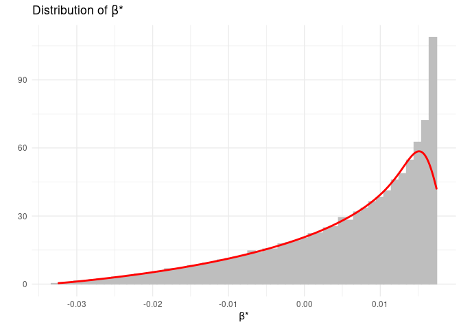
We can create the histogram and density plot of the omitted variable bias.

bate::dplotbate(OVB$Data)

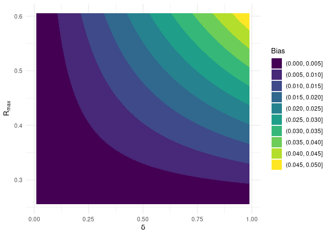
We can also create a contour plot of BATE over the bounded box.

bate::cplotbias(OVB$Data)