Behavioral Economic Easy Demand.
Behavioral Economic (be) Easy (ez) Demand 
![]()
![]()
Behavioral economic demand is gaining in popularity. The motivation behind beezdemand was to create an alternative tool to conduct these analyses. It is meant for researchers to conduct behavioral economic (be) demand the easy (ez) way.
Note About Use
Currently, this version is stable. I encourage you to use it but be aware that, as with any software release, there might be (unknown) bugs present. I’ve tried hard to make this version usable while including the core functionality (described more below). However, if you find issues or would like to contribute, please open an issue on my GitHub page or email me.
Which Model Should I Use?
| Your Situation | Recommended Approach | Learn More |
|---|---|---|
| Single purchase task, individual fits | fit_demand_fixed() | Fixed demand |
| Need group comparisons, random effects | fit_demand_mixed() | Mixed demand |
| Many zeros, two-part modeling needed | fit_demand_hurdle() | Hurdle models |
| Cross-commodity substitution | fit_cp_*() functions | Cross-price models |
For detailed guidance on choosing the right modeling approach, see the model selection guide or vignette("model-selection"). Full documentation is available at the pkgdown site.
Installing beezdemand
CRAN Release (recommended method)
The latest stable version of beezdemand can be found on CRAN and installed using the following command. The first time you install the package, you may be asked to select a CRAN mirror. Simply select the mirror geographically closest to you.
install.packages("beezdemand")

library(beezdemand)
GitHub Release
To install a stable release directly from GitHub, first install and load the devtools package. Then, use install_github to install the package and associated vignette. You don’t need to download anything directly from GitHub, as you should use the following instructions:
install.packages("devtools")

devtools::install_github("brentkaplan/beezdemand", build_vignettes = TRUE)

library(beezdemand)
Using the Package
Example Dataset
An example dataset of responses on an Alcohol Purchase Task is provided. This object is called apt and is located within the beezdemand package. These data are a subset of from the paper by Kaplan & Reed (2018). Participants (id) reported the number of alcoholic drinks (y) they would be willing to purchase and consume at various prices (x; USD). Note the format of the data, which is called “long format”. Long format data are data structured such that repeated observations are stacked in multiple rows, rather than across columns. First, take a look at an extract of the dataset apt, where I’ve subsetted rows 1 through 10 and 17 through 26:
| id | x | y | |
|---|---|---|---|
| 1 | 19 | 0.0 | 10 |
| 2 | 19 | 0.5 | 10 |
| 3 | 19 | 1.0 | 10 |
| 4 | 19 | 1.5 | 8 |
| 5 | 19 | 2.0 | 8 |
| 6 | 19 | 2.5 | 8 |
| 7 | 19 | 3.0 | 7 |
| 8 | 19 | 4.0 | 7 |
| 9 | 19 | 5.0 | 7 |
| 10 | 19 | 6.0 | 6 |
| 17 | 30 | 0.0 | 3 |
| 18 | 30 | 0.5 | 3 |
| 19 | 30 | 1.0 | 3 |
| 20 | 30 | 1.5 | 3 |
| 21 | 30 | 2.0 | 2 |
| 22 | 30 | 2.5 | 2 |
| 23 | 30 | 3.0 | 2 |
| 24 | 30 | 4.0 | 2 |
| 25 | 30 | 5.0 | 2 |
| 26 | 30 | 6.0 | 2 |
The first column contains the row number. The second column contains the id number of the series within the dataset. The third column contains the x values (in this specific dataset, price per drink) and the fourth column contains the associated responses (number of alcoholic drinks purchased at each respective price). There are replicates of id because for each series (or participant), several x values were presented.
Converting from Wide to Long and Vice Versa
For quick conversion, use the built-in convenience function:
long <- pivot_demand_data(wide, format = "long", id_var = "id")
Below is a manual walkthrough using tidyr for when you need more control.
Take for example the format of most datasets that would be exported from a data collection software such as Qualtrics or SurveyMonkey or Google Forms:
## the following code takes the apt data, which are in long format, and converts
## to a wide format that might be seen from data collection software
wide <- tidyr::pivot_wider(apt, names_from = x, values_from = y)
colnames(wide) <- c("id", paste0("price_", seq(1, 16, by = 1)))
knitr::kable(wide[1:5, 1:10])
| id | price_1 | price_2 | price_3 | price_4 | price_5 | price_6 | price_7 | price_8 | price_9 |
|---|---|---|---|---|---|---|---|---|---|
| 19 | 10 | 10 | 10 | 8 | 8 | 8 | 7 | 7 | 7 |
| 30 | 3 | 3 | 3 | 3 | 2 | 2 | 2 | 2 | 2 |
| 38 | 4 | 4 | 4 | 4 | 4 | 4 | 4 | 3 | 3 |
| 60 | 10 | 10 | 8 | 8 | 6 | 6 | 5 | 5 | 4 |
| 68 | 10 | 10 | 9 | 9 | 8 | 8 | 7 | 6 | 5 |
A dataset such as this is referred to as “wide format” because each participant series contains a single row and multiple measurements within the participant are indicated by the columns. This data format is fine for some purposes; however, for beezdemand, data are required to be in “long format” (in the same format as the example data described earlier). In order to convert to the long format, some steps will be required.
First, it is helpful to rename the columns to what the prices actually were. For example, for the purposes of our example dataset, price_1 was $0.00 (free), price_2 was $0.50, price_3 was $1.00, and so on.
## make an object to hold what will be the new column names
newcolnames <- c("id", "0", "0.5", "1", "1.50", "2", "2.50", "3",
                 "4", "5", "6", "7", "8", "9", "10", "15", "20")
## current column names
colnames(wide)
 [1] "id"       "price_1"  "price_2"  "price_3"  "price_4"  "price_5"
 [7] "price_6"  "price_7"  "price_8"  "price_9"  "price_10" "price_11"
[13] "price_12" "price_13" "price_14" "price_15" "price_16"
## replace current column names with new column names
colnames(wide) <- newcolnames

## how new data look (first 5 rows only)
knitr::kable(wide[1:5, ])
| id | 0 | 0.5 | 1 | 1.50 | 2 | 2.50 | 3 | 4 | 5 | 6 | 7 | 8 | 9 | 10 | 15 | 20 |
|---|---|---|---|---|---|---|---|---|---|---|---|---|---|---|---|---|
| 19 | 10 | 10 | 10 | 8 | 8 | 8 | 7 | 7 | 7 | 6 | 6 | 5 | 5 | 4 | 3 | 2 |
| 30 | 3 | 3 | 3 | 3 | 2 | 2 | 2 | 2 | 2 | 2 | 2 | 2 | 1 | 1 | 1 | 1 |
| 38 | 4 | 4 | 4 | 4 | 4 | 4 | 4 | 3 | 3 | 3 | 3 | 2 | 2 | 2 | 0 | 0 |
| 60 | 10 | 10 | 8 | 8 | 6 | 6 | 5 | 5 | 4 | 4 | 3 | 3 | 2 | 2 | 0 | 0 |
| 68 | 10 | 10 | 9 | 9 | 8 | 8 | 7 | 6 | 5 | 5 | 5 | 4 | 4 | 3 | 0 | 0 |
Now we can convert into a long format using some of the helpful functions in the tidyverse package (make sure the package is loaded before trying the commands below).
## using the dataframe 'wide', we specify the key will be 'price', the values
## will be 'consumption', and we will select all columns besides the first ('id')
long <- tidyr::pivot_longer(wide, -id, names_to = "price", values_to = "consumption")

## we'll sort the rows by id
long <- arrange(long, id)

## view the first 20 rows
knitr::kable(long[1:20, ])
| id | price | consumption |
|---|---|---|
| 19 | 0 | 10 |
| 19 | 0.5 | 10 |
| 19 | 1 | 10 |
| 19 | 1.50 | 8 |
| 19 | 2 | 8 |
| 19 | 2.50 | 8 |
| 19 | 3 | 7 |
| 19 | 4 | 7 |
| 19 | 5 | 7 |
| 19 | 6 | 6 |
| 19 | 7 | 6 |
| 19 | 8 | 5 |
| 19 | 9 | 5 |
| 19 | 10 | 4 |
| 19 | 15 | 3 |
| 19 | 20 | 2 |
| 30 | 0 | 3 |
| 30 | 0.5 | 3 |
| 30 | 1 | 3 |
| 30 | 1.50 | 3 |
Two final modifications we will make will be to (1) rename our columns to what the functions in beezdemand will expect to see: id, x, and y, and (2) ensure both x and y are in numeric format.
colnames(long) <- c("id", "x", "y")

long$x <- as.numeric(long$x)
long$y <- as.numeric(long$y)
knitr::kable(head(long))
| id | x | y |
|---|---|---|
| 19 | 0.0 | 10 |
| 19 | 0.5 | 10 |
| 19 | 1.0 | 10 |
| 19 | 1.5 | 8 |
| 19 | 2.0 | 8 |
| 19 | 2.5 | 8 |
The dataset is now “tidy” because: (1) each variable forms a column, (2) each observation forms a row, and (3) each type of observational unit forms a table (in this case, our observational unit is the Alcohol Purchase Task data). To learn more about the benefits of tidy data, readers are encouraged to consult Hadley Wikham’s essay on Tidy Data.
Obtain Descriptive Data
Descriptive statistics at each price (mean, SD, proportion of zeros, min, max) are available via get_descriptive_summary():
desc <- get_descriptive_summary(apt)
desc
Descriptive Summary of Demand Data
===================================

Call:
get_descriptive_summary(data = apt)

Data Summary:
  Subjects: 10
  Prices analyzed: 16

Statistics by Price:
 Price Mean Median   SD PropZeros NAs Min Max
     0  6.8    6.5 2.62       0.0   0   3  10
   0.5  6.8    6.5 2.62       0.0   0   3  10
     1  6.5    6.5 2.27       0.0   0   3  10
   1.5  6.1    6.0 1.91       0.0   0   3   9
     2  5.3    5.5 1.89       0.0   0   2   8
   2.5  5.2    5.0 1.87       0.0   0   2   8
     3  4.8    5.0 1.48       0.0   0   2   7
     4  4.3    4.5 1.57       0.0   0   2   7
     5  3.9    3.5 1.45       0.0   0   2   7
     6  3.5    3.0 1.43       0.0   0   2   6
     7  3.3    3.0 1.34       0.0   0   2   6
     8  2.6    2.5 1.51       0.1   0   0   5
     9  2.4    2.0 1.58       0.1   0   0   5
    10  2.2    2.0 1.32       0.1   0   0   4
    15  1.1    0.5 1.37       0.5   0   0   3
    20  0.8    0.0 1.14       0.6   0   0   3
| Price | Mean | Median | SD | PropZeros | NAs | Min | Max |
|---|---|---|---|---|---|---|---|
| 0 | 6.8 | 6.5 | 2.62 | 0.0 | 0 | 3 | 10 |
| 0.5 | 6.8 | 6.5 | 2.62 | 0.0 | 0 | 3 | 10 |
| 1 | 6.5 | 6.5 | 2.27 | 0.0 | 0 | 3 | 10 |
| 1.5 | 6.1 | 6.0 | 1.91 | 0.0 | 0 | 3 | 9 |
| 2 | 5.3 | 5.5 | 1.89 | 0.0 | 0 | 2 | 8 |
| 2.5 | 5.2 | 5.0 | 1.87 | 0.0 | 0 | 2 | 8 |
| 3 | 4.8 | 5.0 | 1.48 | 0.0 | 0 | 2 | 7 |
| 4 | 4.3 | 4.5 | 1.57 | 0.0 | 0 | 2 | 7 |
| 5 | 3.9 | 3.5 | 1.45 | 0.0 | 0 | 2 | 7 |
| 6 | 3.5 | 3.0 | 1.43 | 0.0 | 0 | 2 | 6 |
| 7 | 3.3 | 3.0 | 1.34 | 0.0 | 0 | 2 | 6 |
| 8 | 2.6 | 2.5 | 1.51 | 0.1 | 0 | 0 | 5 |
| 9 | 2.4 | 2.0 | 1.58 | 0.1 | 0 | 0 | 5 |
| 10 | 2.2 | 2.0 | 1.32 | 0.1 | 0 | 0 | 4 |
| 15 | 1.1 | 0.5 | 1.37 | 0.5 | 0 | 0 | 3 |
| 20 | 0.8 | 0.0 | 1.14 | 0.6 | 0 | 0 | 3 |
A box-and-whisker plot is built in:
plot(desc)
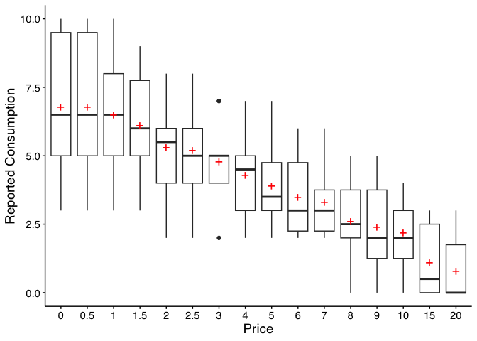
Legacy equivalent:
GetDescriptives(dat = apt, bwplot = TRUE). Seevignette("migration-guide")for details.
Change Data
There are certain instances in which data are to be modified before fitting, for example when using an equation that logarithmically transforms y values. The following function can help with modifying data:
nreplindicates number of replacement 0 values, either as an integer or"all". If this value is an integer,n, then the firstn0s will be replaced.replnumindicates the number that should replace 0 valuesrem0removes all zerosremq0eremoves y value where x (or price) equals 0replfreereplaces where x (or price) equals 0 with a specified number
ChangeData(dat = apt, nrepl = 1, replnum = 0.01, rem0 = FALSE, remq0e = FALSE,
           replfree = NULL)
Identify Unsystematic Responses
Stein et al.’s (2015) algorithm for identifying unsystematic responses is available via check_systematic_demand():
sys_check <- check_systematic_demand(apt)
sys_check
Systematicity Check (demand)
------------------------------
Total patterns: 10
Systematic: 10 ( 100 %)
Unsystematic: 0 ( 0 %)

Use summary() for details, tidy() for per-subject results.
summary(sys_check)
Systematicity Check Summary (demand)
==================================================

Total patterns: 10
Systematic: 10 ( 100 %)
Unsystematic: 0 ( 0 %)

Failures by Criterion:
# A tibble: 4 × 3
  criterion n_fail pct_fail
  <chr>      <int>    <dbl>
1 trend          0        0
2 bounce         0        0
3 reversals      0        0
4 overall        0        0
Legacy equivalent:
CheckUnsystematic(dat = apt, deltaq = 0.025, bounce = 0.1, reversals = 0, ncons0 = 2). Seevignette("migration-guide")for details.
Analyze Demand Data
Obtaining Empirical Measures
Empirical measures (intensity, breakpoint, Omax, Pmax) can be obtained via get_empirical_measures():
emp <- get_empirical_measures(apt)
emp
Empirical Demand Measures
=========================

Call:
get_empirical_measures(data = apt)

Data Summary:
  Subjects: 10
  Subjects with zero consumption: Yes
  Complete cases (no NAs): 6

Empirical Measures:
  id Intensity BP0 BP1 Omaxe Pmaxe
  19        10  NA  20    45    15
  30         3  NA  20    20    20
  38         4  15  10    21     7
  60        10  15  10    24     8
  68        10  15  10    36     9
 106         5   8   7    15     5
 113         6  NA  20    45    15
 142         8  NA  20    60    20
 156         7  20  15    21     7
 188         5  15  10    15     5
| id | Intensity | BP0 | BP1 | Omaxe | Pmaxe |
|---|---|---|---|---|---|
| 19 | 10 | NA | 20 | 45 | 15 |
| 30 | 3 | NA | 20 | 20 | 20 |
| 38 | 4 | 15 | 10 | 21 | 7 |
| 60 | 10 | 15 | 10 | 24 | 8 |
| 68 | 10 | 15 | 10 | 36 | 9 |
Legacy equivalent:
GetEmpirical(dat = apt). Seevignette("migration-guide")for details.
Fitting Demand Curves
The recommended function for fitting individual demand curves is fit_demand_fixed(). It provides a modern S3 interface with summary(), coef(), tidy(), glance(), predict(), and plot() methods.
Key arguments:
equation—"hs"(Hursh & Silberberg, 2008; default) or"koff"(Koffarnus et al., 2015).k— scaling constant. By default, calculated from the sample range + 0.5. Other options:"ind"(individual),"fit"(free parameter),"share"(shared across all series).agg—NULL(individual fits; default),"Mean"(fit to averaged data), or"Pooled"(fit to all data ignoring clustering).
Individual fits (Hursh & Silberberg equation)
fit_hs <- fit_demand_fixed(apt, equation = "hs")
fit_hs
Fixed-Effect Demand Model
==========================

Call:
fit_demand_fixed(data = apt, equation = "hs")

Equation: hs
k: fixed (2)
Subjects: 10 ( 10 converged, 0 failed)

Use summary() for parameter summaries, tidy() for tidy output.
Extract coefficients and tidy output:
head(coef(fit_hs))
# A tibble: 6 × 5
  id    term  estimate estimate_scale term_display
  <chr> <chr>    <dbl> <chr>          <chr>
1 19    q0    10.2     natural        q0
2 19    alpha  0.00205 natural        alpha
3 30    q0     2.81    natural        q0
4 30    alpha  0.00587 natural        alpha
5 38    q0     4.50    natural        q0
6 38    alpha  0.00420 natural        alpha
| id | term | estimate | std.error | statistic | p.value | component | estimate_scale | term_display | estimate_internal |
|---|---|---|---|---|---|---|---|---|---|
| 19 | Q0 | 10.158665 | 0.2685323 | NA | NA | fixed | natural | Q0 | 10.158665 |
| 30 | Q0 | 2.807366 | 0.2257764 | NA | NA | fixed | natural | Q0 | 2.807366 |
| 38 | Q0 | 4.497456 | 0.2146862 | NA | NA | fixed | natural | Q0 | 4.497456 |
| 60 | Q0 | 9.924274 | 0.4591683 | NA | NA | fixed | natural | Q0 | 9.924274 |
| 68 | Q0 | 10.390384 | 0.3290277 | NA | NA | fixed | natural | Q0 | 10.390384 |
| 106 | Q0 | 5.683566 | 0.3002817 | NA | NA | fixed | natural | Q0 | 5.683566 |
| 113 | Q0 | 6.195949 | 0.1744096 | NA | NA | fixed | natural | Q0 | 6.195949 |
| 142 | Q0 | 6.171990 | 0.6408575 | NA | NA | fixed | natural | Q0 | 6.171990 |
| 156 | Q0 | 8.348973 | 0.4105617 | NA | NA | fixed | natural | Q0 | 8.348973 |
| 188 | Q0 | 6.303639 | 0.5636959 | NA | NA | fixed | natural | Q0 | 6.303639 |
Koffarnus equation
fit_koff <- fit_demand_fixed(apt, equation = "koff")
fit_koff
Fixed-Effect Demand Model
==========================

Call:
fit_demand_fixed(data = apt, equation = "koff")

Equation: koff
k: fixed (2)
Subjects: 10 ( 10 converged, 0 failed)

Use summary() for parameter summaries, tidy() for tidy output.
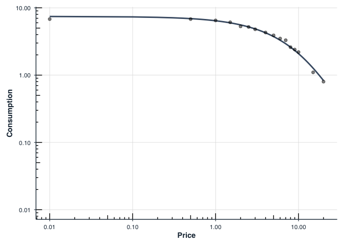
Mean curve
fit_mean <- fit_demand_fixed(apt, equation = "hs", agg = "Mean")
fit_mean
Fixed-Effect Demand Model
==========================

Call:
fit_demand_fixed(data = apt, equation = "hs", agg = "Mean")

Equation: hs
k: fixed (2)
Aggregation: Mean
Subjects: 1 ( 1 converged, 0 failed)

Use summary() for parameter summaries, tidy() for tidy output.
Shared k
fit_share <- fit_demand_fixed(apt, equation = "hs", k = "share")
Beginning search for best-starting k

Best k found at 0.93813356574003 = err: 0.744881846162718

Searching for shared K, this can take a while...
fit_share
Fixed-Effect Demand Model
==========================

Call:
fit_demand_fixed(data = apt, equation = "hs", k = "share")

Equation: hs
k: share
Subjects: 10 ( 10 converged, 0 failed)

Use summary() for parameter summaries, tidy() for tidy output.
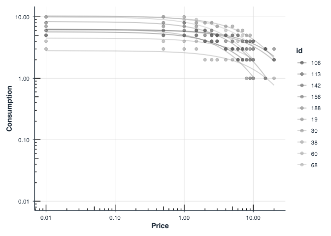
Plotting Demand Curves
All fit_demand_fixed() results support plot():
plot(fit_hs, type = "individual", x_trans = "log10")
Free is shown as `0.01` for purposes of plotting.
plot(fit_mean, x_trans = "log10")
Free is shown as `0.01` for purposes of plotting.
Legacy equivalent: The
FitCurves()+PlotCurves()workflow is still available for backward compatibility. Seevignette("migration-guide")for transitioning fromFitCurves()tofit_demand_fixed().
Compare Values of $\alpha$ and $Q_0$ via Extra Sum-of-Squares F-Test
For mixed-effects group comparisons, consider
fit_demand_mixed()with group factors. Seevignette("group-comparisons").
When one has multiple groups, it may be beneficial to compare whether separate curves are preferred over a single curve. This is accomplished by the Extra Sum-of-Squares F-test. This function (using the argument compare) will determine whether a single $\alpha$ or a single $Q_0$ is better than multiple $\alpha$s or $Q_0$s. A single curve will be fit, the residual deviations calculated and those residuals are compared to residuals obtained from multiple curves. A resulting F statistic will be reporting along with a p value.
## setting the seed initializes the random number generator so results will be
## reproducible
set.seed(1234)

## manufacture random grouping
apt$group <- NA
apt[apt$id %in% sample(unique(apt$id), length(unique(apt$id))/2), "group"] <- "a"
apt$group[is.na(apt$group)] <- "b"

## take a look at what the new groupings look like in long form
knitr::kable(apt[1:20, ])
| id | x | y | group |
|---|---|---|---|
| 19 | 0.0 | 10 | a |
| 19 | 0.5 | 10 | a |
| 19 | 1.0 | 10 | a |
| 19 | 1.5 | 8 | a |
| 19 | 2.0 | 8 | a |
| 19 | 2.5 | 8 | a |
| 19 | 3.0 | 7 | a |
| 19 | 4.0 | 7 | a |
| 19 | 5.0 | 7 | a |
| 19 | 6.0 | 6 | a |
| 19 | 7.0 | 6 | a |
| 19 | 8.0 | 5 | a |
| 19 | 9.0 | 5 | a |
| 19 | 10.0 | 4 | a |
| 19 | 15.0 | 3 | a |
| 19 | 20.0 | 2 | a |
| 30 | 0.0 | 3 | b |
| 30 | 0.5 | 3 | b |
| 30 | 1.0 | 3 | b |
| 30 | 1.5 | 3 | b |
## in order for this to run, you will have had to run the code immediately
## preceeding (i.e., the code to generate the groups)
ef <- ExtraF(dat = apt, equation = "koff", k = 2, groupcol = "group", verbose = TRUE)
Null hypothesis: alpha same for all data sets

Alternative hypothesis: alpha different for each data set

Conclusion: fail to reject the null hypothesis

F(1,156) = 0.0298, p = 0.8631
A summary table (broken up here for ease of display) will be created when the option verbose = TRUE. This table can be accessed as the dfres object resulting from ExtraF. In the example above, we can access this summary table using ef$dfres:
| Group | Q0d | K | R2 | Alpha |
|---|---|---|---|---|
| Shared | NA | NA | NA | NA |
| a | 8.489634 | 2 | 0.6206444 | 0.0040198 |
| b | 5.848119 | 2 | 0.6206444 | 0.0040198 |
| Not Shared | NA | NA | NA | NA |
| a | 8.503442 | 2 | 0.6448801 | 0.0040518 |
| b | 5.822075 | 2 | 0.5242825 | 0.0039376 |
Fitted Measures
| Group | N | AbsSS | SdRes |
|---|---|---|---|
| Shared | NA | NA | NA |
| a | 160 | 387.0945 | 1.570213 |
| b | 160 | 387.0945 | 1.570213 |
| Not Shared | NA | NA | NA |
| a | 80 | 249.2764 | 1.787695 |
| b | 80 | 137.7440 | 1.328890 |
Uncertainty and Model Information
| Group | EV | Omaxd | Pmaxd |
|---|---|---|---|
| Shared | NA | NA | NA |
| a | 0.8795301 | 22.63159 | 8.453799 |
| b | 0.8795301 | 22.63159 | 12.272265 |
| Not Shared | NA | NA | NA |
| a | 0.8725741 | 22.45260 | 8.373320 |
| b | 0.8978945 | 23.10414 | 12.584550 |
Derived Measures
| Group | Omaxa | Notes |
|---|---|---|
| Shared | NA | NA |
| a | 22.63190 | converged |
| b | 22.63190 | converged |
| Not Shared | NA | NA |
| a | 22.45291 | converged |
| b | 23.10445 | converged |
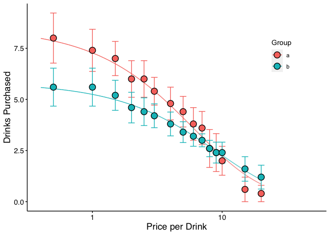
Convergence and Summary Information
When verbose = TRUE, objects from the result can be used in subsequent graphing. The following code generates a plot of our two groups. We can use the predicted values already generated from the ExtraF function by accessing the newdat object. In the example above, we can access these predicted values using ef$newdat. Note that we keep the linear scaling of y given we used Koffarnus et al. (2015)’s equation fitted to the data.
## be sure that you've loaded the tidyverse package (e.g., library(tidyverse))
ggplot(apt, aes(x = x, y = y, group = group)) +
  ## the predicted lines from the sum of squares f-test can be used in subsequent
  ## plots by calling data = ef$newdat
  geom_line(aes(x = x, y = y, group = group, color = group),
            data = ef$newdat[ef$newdat$x >= .1, ]) +
  stat_summary(fun.data = "mean_se", aes(color = group),
               geom = "errorbar", orientation = "x", width = 0) +
  stat_summary(fun = "mean", aes(fill = group), geom = "point", shape = 21,
               color = "black", stroke = .75, size = 4, orientation = "x") +
  scale_x_continuous(limits = c(.4, 50), breaks = c(.1, 1, 10, 100)) +
  coord_trans(x = "log10") +
  scale_color_discrete(name = "Group") +
  scale_fill_discrete(name = "Group") +
  labs(x = "Price per Drink", y = "Drinks Purchased") +
  theme(legend.position = c(.85, .75)) +
  ## theme_apa is a beezdemand function used to change the theme in accordance
  ## with American Psychological Association style
  theme_apa()
Cross-Price Demand Models
In addition to classic purchase-task analyses, beezdemand now includes functions for cross-price demand modeling. These tools help you check for unsystematic data, fit nonlinear or linear/mixed-effects cross-price models, and visualize the results.
Key functions:
check_unsystematic_cp()— identify unsystematic cross-price patterns.fit_cp_nls()— fit nonlinear cross-price models (e.g., exponentiated form).fit_cp_linear()— fit linear and mixed-effects cross-price models.- S3 methods:
summary(),plot(),glance(),tidy().
Minimal example (using the included ETM dataset):
library(dplyr)
data(etm, package = "beezdemand")

# Focus on one product/id and check for unsystematic responding
ex <- etm |> filter(group %in% "E-Cigarettes", id %in% 1)
check_unsystematic_cp(ex)

# Nonlinear cross-price model (exponentiated form)
fit_nls <- fit_cp_nls(ex, equation = "exponentiated", return_all = TRUE)
summary(fit_nls)
plot(fit_nls, x_trans = "log10")
Linear mixed-effects cross-price model across all participants:
fit_mixed <- fit_cp_linear(
  etm,
  type = "mixed",
  log10x = TRUE,
  group_effects = "interaction",
  return_all = TRUE
)
summary(fit_mixed)
plot(fit_mixed, x_trans = "log10", pred_type = "all")
See the vignette “How to Use Cross-Price Demand Model Functions” for a full walkthrough of data structure, modeling options, visualization, and post-hoc comparisons.
Mixed-Effects Demand Models
beezdemand also supports nonlinear mixed-effects demand models to estimate subject-level parameters (e.g., Q0 and alpha) while modeling fixed effects of conditions (e.g., dose, drug). The zben equation form pairs well with the included LL4 transformation to handle zeros and wide dynamic ranges.
Key functions:
fit_demand_mixed()— fit mixed-effects demand models vianlme.ll4()/ll4_inv()— transform and inverse-transform consumption.- Plotting and predictions via
plot()/predict()onbeezdemand_nlmeobjects. - Post-hoc summaries with
get_demand_param_emms()and comparisons usingget_demand_comparisons().
Minimal example (using the included nonhuman dataset ko):
library(dplyr)
data(ko, package = "beezdemand")

# Fit zben form on LL4-transformed consumption with two factors
fit_nlme <- fit_demand_mixed(
  data = ko,
  y_var = "y_ll4",
  x_var = "x",
  id_var = "monkey",
  factors = c("drug", "dose"),
  equation_form = "zben"
)
print(fit_nlme)

# Plot on the natural (back-transformed) scale
plot(
  fit_nlme,
  inv_fun = ll4_inv,
  x_trans = "pseudo_log",
  y_trans = "pseudo_log"
)
For more details, see the “Mixed-Effects Demand Modeling with beezdemand” vignette, which covers starting values, fixed/random effects, and post-hoc analyses of parameter estimates.
Learn More About Functions
To learn more about a function and what arguments it takes, type “?” in front of the function name.
## Modern interface (recommended)
?fit_demand_fixed
?get_empirical_measures
?get_descriptive_summary
?check_systematic_demand

## Legacy interface (still available)
?FitCurves
?CheckUnsystematic
Acknowledgments
Shawn P. Gilroy, Contributor GitHub
Derek D. Reed, Applied Behavioral Economics Laboratory
Mikhail N. Koffarnus, Addiction Recovery Research Center
Steven R. Hursh, Institutes for Behavior Resources, Inc.
Paul E. Johnson, Center for Research Methods and Data Analysis, University of Kansas
Peter G. Roma, Institutes for Behavior Resources, Inc.
W. Brady DeHart, Addiction Recovery Research Center
Michael Amlung, Cognitive Neuroscience of Addictions Laboratory
Special thanks to the following people who helped provide feedback on this document:
Alexandra M. Mellis
Mr. Jeremiah “Downtown Jimbo Brown” Brown
Gideon Naudé
LLM Docs
The package publishes machine-readable documentation for use with AI coding assistants and RAG systems:
llms.txt— canonical entry point for LLMs, published at: https://brentkaplan.github.io/beezdemand/llms.txt- Context7 — a
context7.jsonat the repo root configures Context7 indexing. Use/brentkaplan/beezdemandas the library ID in Context7-enabled tools. - Docs map — a chunkable reference at
inst/llm/docs-map.mdsummarises workflows, data format, and key functions for RAG ingestion.
Recommended Readings
Reed, D. D., Niileksela, C. R., & Kaplan, B. A. (2013). Behavioral economics: A tutorial for behavior analysts in practice. Behavior Analysis in Practice, 6 (1), 34–54. https://doi.org/10.1007/BF03391790
Reed, D. D., Kaplan, B. A., & Becirevic, A. (2015). Basic research on the behavioral economics of reinforcer value. In Autism Service Delivery (pp. 279-306). Springer New York. https://doi.org/10.1007/978-1-4939-2656-5_10
Hursh, S. R., & Silberberg, A. (2008). Economic demand and essential value. Psychological Review, 115 (1), 186-198. https://doi.org/10.1037/0033-295X.115.1.186
Koffarnus, M. N., Franck, C. T., Stein, J. S., & Bickel, W. K. (2015). A modified exponential behavioral economic demand model to better describe consumption data. Experimental and Clinical Psychopharmacology, 23 (6), 504-512. https://doi.org/10.1037/pha0000045
Stein, J. S., Koffarnus, M. N., Snider, S. E., Quisenberry, A. J., & Bickel, W. K. (2015). Identification and management of nonsystematic purchase task data: Toward best practice. Experimental and Clinical Psychopharmacology 23 (5), 377-386. https://doi.org/10.1037/pha0000020
Hursh, S. R., Raslear, T. G., Shurtleff, D., Bauman, R., & Simmons, L. (1988). A cost‐benefit analysis of demand for food. Journal of the Experimental Analysis of Behavior, 50 (3), 419-440. https://doi.org/10.1901/jeab.1988.50-419
Kaplan, B. A., Franck, C. T., McKee, K., Gilroy, S. P., & Koffarnus, M. N. (2021). Applying mixed-effects modeling to behavioral economic demand: An introduction. Perspectives on Behavior Science, 44 (2), 333–358. https://doi.org/10.1007/s40614-021-00299-7
Koffarnus, M. N., Kaplan, B. A., Franck, C. T., Rzeszutek, M. J., & Traxler, H. K. (2022). Behavioral economic demand modeling chronology, complexities, and considerations: Much ado about zeros. Behavioural Processes, 199, 104646. https://doi.org/10.1016/j.beproc.2022.104646
Reed, D. D., Kaplan, B. A., & Gilroy, S. P. (2025). Handbook of Operant Behavioral Economics: Demand, Discounting, Methods, and Applications (1st ed.). Academic Press. https://shop.elsevier.com/books/handbook-of-operant-behavioral-economics/reed/978-0-323-95745-8
Kaplan, B. A. (2025). Quantitative models of operant demand. In D. D. Reed, B. A. Kaplan, & S. P. Gilroy (Eds.), Handbook of Operant Behavioral Economics: Demand, Discounting, Methods, and Applications (1st ed.). Academic Press. https://shop.elsevier.com/books/handbook-of-operant-behavioral-economics/reed/978-0-323-95745-8
Kaplan, B. A., & Reed, D. D. (2025). shinybeez: A Shiny app for behavioral economic easy demand and discounting. Journal of the Experimental Analysis of Behavior. https://doi.org/10.1002/jeab.70000
Rzeszutek, M. J., Regnier, S. D., Franck, C. T., & Koffarnus, M. N. (2025). Overviewing the exponential model of demand and introducing a simplification that solves issues of span, scale, and zeros. Experimental and Clinical Psychopharmacology.
Rzeszutek, M. J., Regnier, S. D., Kaplan, B. A., Traxler, H. K., Stein, J. S., Tomlinson, D., & Koffarnus, M. N. (2025). Identification and management of nonsystematic cross-commodity data: Toward best practice. Experimental and Clinical Psychopharmacology. In press.