Bayesian Neural Network with 'Stan'.

bnns

The bnns package provides tools to fit Bayesian Neural Networks (BNNs) for regression and classification problems. It is designed to be flexible, supporting various network architectures, activation functions, and output types, making it suitable for both simple and complex data analysis tasks.

Features

• Support for multi-layer neural networks with customizable architecture.
• Choice of activation functions (e.g., sigmoid, ReLU, tanh).
• Outputs for regression (continuous response) and classification (binary and multiclass).
• Choice of prior distributions for weights, biases and sigma (for regression).
• Bayesian inference, providing posterior distributions for predictions and parameters.
• Applications in domains such as clinical trials, predictive modeling, and more.

Installation (stable CRAN version)

To install the bnns package from CRAN, use the following:

install.packages("bnns")

Installation (development version)

To install the bnns package from GitHub, use the following:

# Install devtools if not already installed
if (!requireNamespace("devtools", quietly = TRUE)) {
  install.packages("devtools")
}

# Install bnns
devtools::install_github("swarnendu-stat/bnns")

Getting Started

1. Iris Data

We use the iris data for regression:

head(iris)
#>   Sepal.Length Sepal.Width Petal.Length Petal.Width Species
#> 1          5.1         3.5          1.4         0.2  setosa
#> 2          4.9         3.0          1.4         0.2  setosa
#> 3          4.7         3.2          1.3         0.2  setosa
#> 4          4.6         3.1          1.5         0.2  setosa
#> 5          5.0         3.6          1.4         0.2  setosa
#> 6          5.4         3.9          1.7         0.4  setosa

2. Fit a BNN Model

To fit a Bayesian Neural Network:

library(bnns)

iris_bnn <- bnns(Sepal.Length ~ -1 + ., data = iris, L = 1, act_fn = 3, nodes = 4, out_act_fn = 1, chains = 1)

3. Model Summary

Summarize the fitted model:

summary(iris_bnn)
#> Call:
#> bnns.default(formula = Sepal.Length ~ -1 + ., data = iris, L = 1, 
#>     nodes = 4, act_fn = 3, out_act_fn = 1, chains = 1)
#> 
#> Data Summary:
#> Number of observations: 150 
#> Number of features: 6 
#> 
#> Network Architecture:
#> Number of hidden layers: 1 
#> Nodes per layer: 4 
#> Activation functions: 3 
#> Output activation function: 1 
#> 
#> Posterior Summary (Key Parameters):
#>                mean      se_mean         sd       2.5%         25%        50%
#> w_out[1]  0.8345667 0.0728930420 0.65030179 -0.4150176  0.38054488  0.7769148
#> w_out[2] -0.3719132 0.4067431773 0.96605220 -1.7062097 -1.03225732 -0.7365945
#> w_out[3]  0.4783495 0.1965466796 0.86504113 -1.2350476  0.02944919  0.5634587
#> w_out[4]  0.4537029 0.3334670001 0.89069977 -1.3791675  0.09313077  0.5518418
#> b_out     2.2082591 0.0614548175 1.18859472 -0.1036760  1.38416657  2.2072194
#> sigma     0.3015085 0.0004831093 0.01804107  0.2693205  0.28895030  0.3013415
#>                75%     97.5%       n_eff      Rhat
#> w_out[1] 1.2478028 2.1730066   79.589862 1.0254227
#> w_out[2] 0.4680286 1.7548944    5.641059 1.3136052
#> w_out[3] 1.0454306 2.0448172   19.370556 1.1335888
#> w_out[4] 1.0281249 2.0733860    7.134392 1.1997484
#> b_out    3.1573563 4.2214829  374.072451 1.0016806
#> sigma    0.3128869 0.3386066 1394.549362 0.9988699
#> 
#> Model Fit Information:
#> Iterations: 1000 
#> Warmup: 200 
#> Thinning: 1 
#> Chains: 1 
#> 
#> Predictive Performance:
#> RMSE (training): 0.2821305 
#> MAE (training): 0.2234606 
#> 
#> Notes:
#> Check convergence diagnostics for parameters with high R-hat values.

4. Predictions

Make predictions using the trained model:

pred <- predict(iris_bnn)

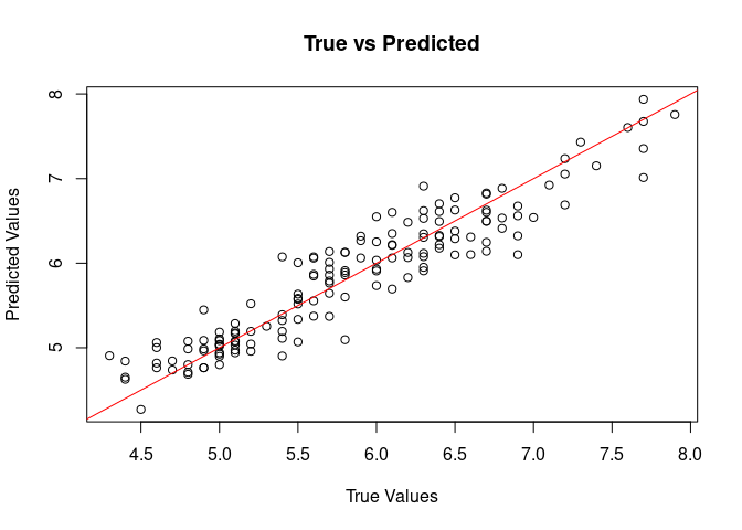
5. Visualization

Visualize true vs predicted values for regression:

plot(iris$Sepal.Length, rowMeans(pred), main = "True vs Predicted", xlab = "True Values", ylab = "Predicted Values")
abline(0, 1, col = "red")

Applications

Regression Example (with custom priors)

Use bnns for regression analysis to model continuous outcomes, such as predicting patient biomarkers in clinical trials.

model <- bnns(Sepal.Length ~ -1 + .,
  data = iris, L = 1, act_fn = 3, nodes = 4,
  out_act_fn = 1, chains = 1,
  prior_weights = list(dist = "uniform", params = list(alpha = -1, beta = 1)),
  prior_bias = list(dist = "cauchy", params = list(mu = 0, sigma = 2.5)),
  prior_sigma = list(dist = "inv_gamma", params = list(alpha = 1, beta = 1))
)

Classification Example

For binary or multiclass classification, set the out_act_fn to 2 (binary) or 3 (multiclass). For example:

# Simulate binary classification data
df <- data.frame(
  x1 = runif(10), x2 = runif(10),
  y = sample(0:1, 10, replace = TRUE)
)

# Fit a binary classification BNN
model <- bnns(y ~ -1 + x1 + x2,
  data = df, L = 2, nodes = c(16, 8),
  act_fn = c(3, 2), out_act_fn = 2, iter = 1e2,
  warmup = 5e1, chains = 1
)

Clinical Trial Applications

Explore posterior probabilities to estimate treatment effects or success probabilities in clinical trials. For example, calculate the posterior probability of achieving a clinically meaningful outcome in a given population.

Documentation

• Detailed vignettes are available to guide through various applications of the package.
• See help(bnns) for more information about the bnns function and its arguments.

Contributing

Contributions are welcome! Please raise issues or submit pull requests on GitHub.

License

This package is licensed under the Apache License. See LICENSE for details.