Description

Decision-Theoretic Causal Diagnostics via Le Cam Deficiency.

Description

Implements Le Cam deficiency theory for causal inference, as described in Akdemir (2026) <doi:10.5281/zenodo.18367347>. Provides theorem-backed bounds together with computable proxy diagnostics for information loss from confounding, selection bias, and distributional shift. Supports continuous, binary, count, survival, and competing risks outcomes. Key features include propensity-score total-variation deficiency proxies, negative control diagnostics, policy regret bounds, and sensitivity analysis via confounding frontiers.

README.md

cran.r-project.org

causaldef

causaldef implements Le Cam deficiency theory for causal inference, providing quantitative bounds on information loss from confounding, selection bias, and distributional shift.

Unlike traditional sensitivity analysis which focuses on “how much bias” exists, causaldef answers the decision-theoretic question: “how much regret” might we incur by acting on this evidence?

Key Concept: Deficiency (δ)

The deficiency δ is a theoretical measure of the information gap between your observational data and a perfect randomized trial. In practice, causaldef provides a computable proxy $\widehat{\delta}$ based on propensity-score TV balance (PS-TV), which is informative about overlap/positivity and residual confounding risk.

For bounded utilities with range $M$ (max minus min), the manuscript provides:

a regret transfer penalty (upper bound term) of $M\cdot\delta$ , and
a minimax safety floor (lower bound) of $(M/2)\cdot\delta$ .

policy_regret_bound() reports both quantities.

Scientific Contract

causaldef is theory-forward, but not every exported quantity is the same kind of object. The package distinguishes:

Theorem-backed quantities: closed-form or theorem-aligned utilities such as policy_regret_bound(), policy_regret_bound_vc(), confounding_frontier(), sharp_lower_bound(), and wasserstein_deficiency_gaussian()
Computable deficiency proxies: estimate_deficiency() currently returns a PS-TV proxy, not a generic nonparametric estimator of the exact Le Cam deficiency
Sensitivity diagnostics: nc_diagnostic() combines an observable residual-association diagnostic with a user-supplied alignment parameter kappa
Experimental heuristics: some specialized modules expose effect estimates together with heuristic proxy scores; those help with exploration, but they should not be read as exact deficiency estimators unless stated explicitly

Installation

You can install the development version of causaldef from GitHub with:

# install.packages("devtools")
devtools::install_github("denizakdemir/causaldef")

Core Features

Deficiency proxies:estimate_deficiency() (PS-TV overlap/balance proxy)
Policy regret bounds:policy_regret_bound() (transfer penalty
- minimax floor)
Negative control diagnostics:nc_diagnostic() (falsification and bounds)
Sensitivity analysis:confounding_frontier() (linear-Gaussian confounding frontier)
Survival + competing risks:causal_spec_survival(), causal_spec_competing()

Example 1: Basic Deficiency Estimation

library(causaldef)
set.seed(42)

# Simulate confounded data (W satisfies back-door criterion)
n <- 500
W <- rnorm(n)
A <- rbinom(n, 1, plogis(0.5 * W))
Y <- 1 + 2 * A + W + rnorm(n)
df <- data.frame(W = W, A = A, Y = Y)

# 1. Define the causal problem
spec <- causal_spec(
  data = df,
  treatment = "A",
  outcome = "Y",
  covariates = "W"
)
#> ✔ Created causal specification: n=500, 1 covariate(s)

# 2. Estimate a deficiency proxy (PS-TV) for different strategies
results <- estimate_deficiency(
  spec, 
  methods = c("unadjusted", "iptw", "aipw"),
  n_boot = 100
)
#> ℹ Estimating deficiency: unadjusted
#> ℹ Estimating deficiency: iptw
#> ℹ Estimating deficiency: aipw

print(results)
#> 
#> -- Deficiency Proxy Estimates (PS-TV) ------
#> 
#>      Method  Delta     SE               CI            Quality
#>  unadjusted 0.1190 0.0230 [0.1048, 0.1982] Insufficient (Red)
#>        iptw 0.0212 0.0099 [0.0142, 0.0537]  Excellent (Green)
#>        aipw 0.0212 0.0087 [0.0154, 0.0483]  Excellent (Green)
#> Note: delta is a propensity-score TV proxy (overlap/balance diagnostic).
#> 
#> Best method: iptw (delta = 0.0212 )

Interpretation: Unadjusted $\widehat{\delta}\approx$ 0.119; after IPTW/AIPW, $\widehat{\delta}\approx$ 0.021.

Example 2: Policy Regret Bounds

If we use this evidence to make a policy decision (e.g., approve a drug), what is the worst-case loss?

# Calculate bounds for a utility range of [0, 1]
bounds <- policy_regret_bound(results, utility_range = c(0, 1), method = "aipw")
#> ℹ Transfer penalty: 0.0212 (delta = 0.0212)

print(bounds)
#> 
#> -- Policy Regret Bounds -------------------------------------------------
#> 
#> * Deficiency delta: 0.0212 
#> * Delta mode: point 
#> * Delta method: aipw 
#> * Delta selection: pre-specified method 
#> * Utility range: [0, 1]
#> * Transfer penalty: 0.0212 (additive regret upper bound)
#> * Minimax floor: 0.0106 (worst-case lower bound)
#> 
#> Note: this is a plug-in bound using a deficiency proxy rather than an identified exact deficiency.
#> 
#> Interpretation: Transfer penalty is 2.1 % of utility range given delta
plot(bounds, type = "safety_curve")
#> Warning: Ignoring unknown parameters: linewidth
#> Warning: Ignoring unknown parameters: linewidth

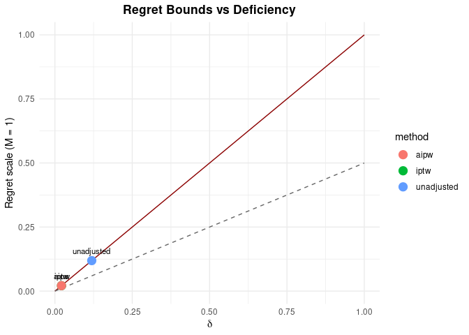
The plug-in transfer penalty is 0.0212 on a 0–1 utility scale; the minimax safety floor is 0.0106.

Example 3: Negative Control Diagnostic

Check if the “Adjusted” strategy actually removes confounding using a negative control outcome $Y_{nc}$ (known to be unaffected by treatment).

# Add a negative control to simulation
df$Y_nc <- W + rnorm(n) # Correlated with W (confounder) but not A

spec_nc <- causal_spec(
  data = df, 
  treatment = "A", 
  outcome = "Y",
  covariates = "W",
  negative_control = "Y_nc"
)
#> ✔ Created causal specification: n=500, 1 covariate(s)

# Run diagnostic
nc_test <- nc_diagnostic(spec_nc, method = "iptw")
#> ℹ Using kappa = 1 (conservative). Consider domain-specific estimation or sensitivity analysis via kappa_range.
#> ✔ No evidence against causal assumptions (p = 0.8607 )
print(nc_test)
#> 
#> -- Negative Control Diagnostic ----------------------------------------
#> 
#> * screening statistic (weighted corr): 0.0089 
#> * delta_NC (association proxy): 0.0089 
#> * delta bound (under kappa alignment): 0.0089 (kappa = 1 )
#> * screening p-value: 0.8607 
#> * screening method: weighted_permutation_correlation 
#> 
#> RESULT: NOT REJECTED. This is a screening result, not proof that confounding is absent.
#> NOTE: Your effect estimate must exceed the Noise Floor (delta_bound) to be meaningful.

Here, the test does not reject (p = 0.861), and the observable proxy is $\widehat{\delta}_{NC}\approx$ 0.009.

Example 4: Survival Analysis (HCT)

data(hct_outcomes)

# Create an explicit 0/1 event indicator (any non-censor event)
hct <- hct_outcomes
hct$event_any <- as.integer(hct$event_status != "Censored")

spec_surv <- causal_spec_survival(
  data = hct,
  treatment = "conditioning_intensity",
  time = "time_to_event",
  event = "event_any",
  covariates = c("age", "disease_status", "kps", "donor_type"),
  estimand = "RMST",
  horizon = 24
)
#> ✔ Created survival causal specification: n=800, 677 events

def_surv <- estimate_deficiency(spec_surv, methods = c("unadjusted", "cox_iptw"), n_boot = 50)
#> ℹ Inferred treatment value: Reduced
#> ℹ Estimating deficiency: unadjusted
#> ℹ Estimating deficiency: cox_iptw
#> ! Weighted Cox model failed: could not find function "deparse1"
#> ! Weighted Cox model failed: could not find function "deparse1"
#> ! Weighted Cox model failed: could not find function "deparse1"
#> ! Weighted Cox model failed: could not find function "deparse1"
#> ! Weighted Cox model failed: could not find function "deparse1"
#> ! Weighted Cox model failed: could not find function "deparse1"
#> ! Weighted Cox model failed: could not find function "deparse1"
#> ! Weighted Cox model failed: could not find function "deparse1"
#> ! Weighted Cox model failed: could not find function "deparse1"
#> ! Weighted Cox model failed: could not find function "deparse1"
#> ! Weighted Cox model failed: could not find function "deparse1"
#> ! Weighted Cox model failed: could not find function "deparse1"
#> ! Weighted Cox model failed: could not find function "deparse1"
#> ! Weighted Cox model failed: could not find function "deparse1"
#> ! Weighted Cox model failed: could not find function "deparse1"
#> ! Weighted Cox model failed: could not find function "deparse1"
#> ! Weighted Cox model failed: could not find function "deparse1"
#> ! Weighted Cox model failed: could not find function "deparse1"
#> ! Weighted Cox model failed: could not find function "deparse1"
#> ! Weighted Cox model failed: could not find function "deparse1"
#> ! Weighted Cox model failed: could not find function "deparse1"
#> ! Weighted Cox model failed: could not find function "deparse1"
#> ! Weighted Cox model failed: could not find function "deparse1"
#> ! Weighted Cox model failed: could not find function "deparse1"
#> ! Weighted Cox model failed: could not find function "deparse1"
#> ! Weighted Cox model failed: could not find function "deparse1"
#> ! Weighted Cox model failed: could not find function "deparse1"
#> ! Weighted Cox model failed: could not find function "deparse1"
#> ! Weighted Cox model failed: could not find function "deparse1"
#> ! Weighted Cox model failed: could not find function "deparse1"
#> ! Weighted Cox model failed: could not find function "deparse1"
#> ! Weighted Cox model failed: could not find function "deparse1"
#> ! Weighted Cox model failed: could not find function "deparse1"
#> ! Weighted Cox model failed: could not find function "deparse1"
#> ! Weighted Cox model failed: could not find function "deparse1"
#> ! Weighted Cox model failed: could not find function "deparse1"
#> ! Weighted Cox model failed: could not find function "deparse1"
#> ! Weighted Cox model failed: could not find function "deparse1"
#> ! Weighted Cox model failed: could not find function "deparse1"
#> ! Weighted Cox model failed: could not find function "deparse1"
#> ! Weighted Cox model failed: could not find function "deparse1"
#> ! Weighted Cox model failed: could not find function "deparse1"
#> ! Weighted Cox model failed: could not find function "deparse1"
#> ! Weighted Cox model failed: could not find function "deparse1"
#> ! Weighted Cox model failed: could not find function "deparse1"
#> ! Weighted Cox model failed: could not find function "deparse1"
#> ! Weighted Cox model failed: could not find function "deparse1"
#> ! Weighted Cox model failed: could not find function "deparse1"
#> ! Weighted Cox model failed: could not find function "deparse1"
#> ! Weighted Cox model failed: could not find function "deparse1"
#> ! Weighted Cox model failed: could not find function "deparse1"
print(def_surv)
#> 
#> -- Deficiency Proxy Estimates (PS-TV) ------
#> 
#>      Method  Delta     SE               CI            Quality
#>  unadjusted 0.3030 0.0606 [0.2369, 0.4526] Insufficient (Red)
#>    cox_iptw 0.0076 0.0047 [0.0066, 0.0247]  Excellent (Green)
#> Note: delta is a propensity-score TV proxy (overlap/balance diagnostic).
#> 
#> Best method: cox_iptw (delta = 0.0076 )

bounds_surv <- policy_regret_bound(def_surv, utility_range = c(0, 24), method = "cox_iptw")
#> ℹ Transfer penalty: 0.1823 (delta = 0.0076)
print(bounds_surv)
#> 
#> -- Policy Regret Bounds -------------------------------------------------
#> 
#> * Deficiency delta: 0.0076 
#> * Delta mode: point 
#> * Delta method: cox_iptw 
#> * Delta selection: pre-specified method 
#> * Utility range: [0, 24]
#> * Transfer penalty: 0.1823 (additive regret upper bound)
#> * Minimax floor: 0.0911 (worst-case lower bound)
#> 
#> Note: this is a plug-in bound using a deficiency proxy rather than an identified exact deficiency.
#> 
#> Interpretation: Transfer penalty is 0.8 % of utility range given delta

Theory

Based on Akdemir (2026), “Constraints on Causal Inference as Experiment Comparison”.

The core theorem links the deficiency $\delta$ (Total Variation distance) to the max-min regret:

$\text{Regret}_{do}(\pi) \leq \text{Regret}_{obs}(\pi) + M\cdot \delta$

Where $M$ is the range of the utility function. In practice, the package often provides plug-in bounds by feeding a computable proxy/estimate (e.g., $\widehat{\delta}$ ) into the regret formula, so the interpretation should track the underlying quantity being supplied.

Citation

@misc{causaldef,
  title = {causaldef: Decision-Theoretic Causal Diagnostics via Le Cam Deficiency},
  author = {Akdemir, Deniz},
  year = {2026},
  doi = {10.5281/zenodo.18367347}
}

r-causaldef

causaldef

Key Concept: Deficiency (δ)

Scientific Contract

Installation

Core Features

Example 1: Basic Deficiency Estimation

Example 2: Policy Regret Bounds

Example 3: Negative Control Diagnostic

Example 4: Survival Analysis (HCT)

Theory

Citation

Version

License

Status

Source

Homepage

Platforms (80)

causaldef

Key Concept: Deficiency (δ)

Scientific Contract

Installation

Core Features

Example 1: Basic Deficiency Estimation

Example 2: Policy Regret Bounds

Example 3: Negative Control Diagnostic

Example 4: Survival Analysis (HCT)

Theory

Citation

Version

License

Status

Source

Homepage

Platforms80 (80)

Platforms (80)