Clinical Publication.
clinpubr: Clinical Publication
![]()
![]()
Overview
clinpubr is an R package designed to streamline the workflow from clinical data processing to publication-ready outputs. It provides tools for clinical data cleaning, significant result screening, and generating tables/figures suitable for medical journals.
Key Features
- Clinical Data Cleaning: Functions to handle missing values, standardize units, convert dates, and clean numerical/categorical variables.
- Result Screening: Screening results of regression and interaction analysis with common variable transformations to identify key findings.
- Publication-Ready Outputs: Generate baseline characteristic tables, forest plots, RCS curves, and other visualizations formatted for medical publications.
Installation
You can install clinpubr from CRAN with:
install.packages("clinpubr")
Optional Dependencies
Some functions require additional packages for full functionality. The package will automatically prompt you to install missing packages when needed. If you want to install the package with all dependencies, you can use:
install.packages("clinpubr", dependencies = TRUE)
Basic Usage
Cleaning Tools
Example 1.1: Generate Data Overview and Cleaning Recommendations
library(clinpubr)

# Sample messy data with various quality issues
messy_data <- data.frame(
  id = 1:15,
  # Numeric with outliers
  bmi = c(
    22.5, 23.1, 24.2, 21.8, 25.0, 23.5, 999, 24.1, 22.9, 23.8,
    21.5, 24.3, 23.0, 22.7, 23.9
  ),
  # Character with case inconsistency
  city = c(
    "Beijing", "BEIJING", "beijing", "Shanghai", "SHANGHAI",
    "Guangzhou", "chengdu", "CHENGDU", "Shenzhen", "shenzhen",
    "Beijing", "Shanghai", "Guangzhou", "Chengdu", "Shenzhen"
  ),
  # Numeric with negative values in predominantly positive
  height = c(
    1.75, 1.80, 1.65, 1.70, 1.85, 1.78, 1.68, 1.72, 1.76, 1.82,
    1.60, 1.62, 1.74, 179, -1
  ),
  # Date with suspicious year
  visit_date = as.Date(c(
    "2020-01-15", "2020-02-20", "2020-03-10", "2019-05-18", "2020-06-22",
    "2018-07-30", "2020-08-12", "2020-09-25", "2020-10-08", "2020-11-15",
    "2020-12-20", "1900-01-01", "2030-02-28", "2020-03-15", "2020-04-20"
  )),
  # Numeric stored as character
  age = c(
    "25", "26", "27", "28", "29", "30", "31", "32", "33", "34",
    "35", "unknown", "36", "37", "38"
  )
)

overview <- data_overview(messy_data)
#> === Data Overview Summary ===
#> Dataset: 15 rows, 6 columns
#>
#> Variable Types:
#>   numeric   : 3 variables
#>   character : 2 variables
#>   date      : 1 variables
#>
#> Found 6 potential quality issues:
#>   numeric_as_character     : 1 cases
#>   outliers                 : 2 cases
#>   negative_in_positive     : 1 cases
#>   suspicious_dates         : 1 cases
#>   case_issues              : 1 cases
#>
#> Recommendations:
#>   - Consider converting these character variables to numeric: age
#>   - Review outliers in these numeric variables: bmi, height
#>   - Numeric variables with mostly positive values but containing negatives: height
#>   - Review suspicious dates (year < 1910 or > current year) in: visit_date
#>   - These character variables have case inconsistency issues: city - consider standardizing to lowercase or uppercase

print(overview$quality_issues$case_issues)
#> $city
#> $city$n_original
#> [1] 11
#>
#> $city$n_normalized
#> [1] 5
#>
#> $city$reduction
#> [1] 6
#>
#> $city$examples
#> $city$examples$beijing
#> [1] "Beijing" "BEIJING" "beijing"
#>
#> $city$examples$shanghai
#> [1] "Shanghai" "SHANGHAI"
#>
#> $city$examples$chengdu
#> [1] "chengdu" "CHENGDU" "Chengdu"
Example 1.2: Screen Multi-Table Cohort by Entry and Anchor Rules
patient <- data.frame(pid = 1:4)
admission <- data.frame(
  pid = c(1, 1, 2, 3, 4),
  vid = c(11, 12, 21, 31, 41),
  admit_day = c(1, 5, 2, 3, 4)
)
diagnosis <- data.frame(
  pid = c(1, 2, 3, 4),
  vid = c(11, 21, 31, 41),
  dx_day = c(1, 2, 3, 4),
  icd = c("I10", "I10", "J18", "I11")
)
lab <- data.frame(
  pid = c(1, 1, 2, 2, 3, 4),
  vid = c(11, 12, 21, 21, 31, 41),
  lab_day = c(1, 5, 2, 5, 3, 4),
  Hb = c(9.8, 10.6, 10.7, 5, 8.9, 9.1)
)

# Keep patients with any I10 diagnosis, then keep records from first Hb > 10 onward, and join tables together
res <- screen_data_list(
  data_list = list(patient = patient, admission = admission, diagnosis = diagnosis, lab = lab),
  entry_expr = any(icd == "I10"),
  entry_level = "patient_id",
  anchor_expr = any(Hb > 10),
  anchor_level = "visit_id",
  anchor_window = "from_first_anchor",
  patient_id_map = "pid",
  visit_id_map = "vid",
  date_map = c(admission = "admit_day", diagnosis = "dx_day", lab = "lab_day"),
  output = "joined"
)

knitr::kable(res)
| patient_id | visit_id | date | icd | Hb |
|---|---|---|---|---|
| 1 | 12 | 5 | NA | 10.6 |
| 2 | 21 | 2 | I10 | 10.7 |
| 2 | 21 | 5 | NA | 5.0 |
Example 1.3: Standardize Values in Medical Records
# Sample messy data
messy_data <- data.frame(values = c("12.3", "0..45", "  67 ", "", "abandon"))
clean_data <- value_initial_cleaning(messy_data$values)
print(clean_data)
#> [1] "12.3"    "0.45"    "67"      NA        "abandon"
Example 1.4: Check Non-numerical Values
# Sample messy data
x <- c("1.2(XXX)", "1.5", "0.82", "5-8POS", "NS", "FULL")
print(check_nonnum(x))
#> [1] "1.2(XXX)" "5-8POS"   "NS"       "FULL"
This function filters out non-numerical values, which helps you choose the appropriate method to handle them.
Example 1.5: Extracting Numerical Values from Text
# Sample messy data
x <- c("1.2(XXX)", "1.5", "0.82", "5-8POS", "NS", "FULL")
print(extract_num(x))
#> [1] 1.20 1.50 0.82 5.00   NA   NA

print(extract_num(x,
  res_type = "first", # Extract the first number
  multimatch2na = TRUE, # Convert illegal multiple matches to NA
  zero_regexp = "NEG|NS", # Convert "NEG" and "NS" (matched using regex) to 0
  max_regexp = "FULL", # Convert "FULL" (matched using regex) to some specified quantile
  max_quantile = 0.95
))
#> [1] 1.20 1.50 0.82   NA 0.00 1.47
Other Cleaning Functions
to_date(): Convert text to date, can handle mixed format.unit_view()andunit_standardize(): Provide a pipeline to standardize conflicting units.cut_by(): Split numerics into factors, offers a variety of splitting options and auto labeling.- And more…
Screening Results to Identify Potential Findings
data(cancer, package = "survival")

# Screening for potential findings with regression models in the cancer dataset
scan_result <- regression_scan(cancer, y = "status", time = "time", save_table = FALSE)
#> Taking all variables as predictors
knitr::kable(scan_result)
| predictor | nvalid | original.HR | original.pval | original.padj | logarithm.HR | logarithm.pval | logarithm.padj | categorized.HR | categorized.pval | categorized.padj | rcs.overall.pval | rcs.overall.padj | rcs.nonlinear.pval | rcs.nonlinear.padj | best.var.trans | |
|---|---|---|---|---|---|---|---|---|---|---|---|---|---|---|---|---|
| 4 | ph.ecog | 227 | 1.6095320 | 0.0000269 | 0.0002154 | NA | NA | NA | NA | 0.0001530 | 0.0012237 | NA | NA | NA | NA | original |
| 6 | pat.karno | 225 | 0.9803456 | 0.0002824 | 0.0011296 | 0.2709544 | 0.0003071 | 0.0015356 | 0.5755627 | 0.0006608 | 0.0026431 | 0.0025848 | 0.0155086 | 0.5908952 | 0.8863427 | original |
| 3 | sex | 228 | 0.5880028 | 0.0014912 | 0.0039766 | NA | NA | NA | 0.5880028 | 0.0014912 | 0.0039766 | NA | NA | NA | NA | categorized |
| 5 | ph.karno | 227 | 0.9836863 | 0.0049579 | 0.0099157 | 0.3184168 | 0.0079468 | 0.0198669 | 0.6352465 | 0.0077670 | 0.0155339 | 0.0128462 | 0.0385385 | 0.2307961 | 0.6848245 | original |
| 2 | age | 228 | 1.0188965 | 0.0418531 | 0.0669650 | 3.0256773 | 0.0466926 | 0.0778209 | 1.1440790 | 0.3910647 | 0.3957558 | 0.0825447 | 0.1650894 | 0.3424123 | 0.6848245 | original |
| 1 | inst | 227 | 0.9903692 | 0.3459838 | 0.4613117 | 0.9292046 | 0.3181432 | 0.3976790 | 0.8384047 | 0.2600040 | 0.3466720 | 0.8175277 | 0.8707131 | 0.9839705 | 0.9839705 | categorized |
| 7 | meal.cal | 181 | 0.9998762 | 0.5929402 | 0.6776459 | 0.9141580 | 0.6128095 | 0.6128095 | 0.8620604 | 0.3957558 | 0.3957558 | 0.8707131 | 0.8707131 | 0.8227256 | 0.9839705 | categorized |
| 8 | wt.loss | 214 | 1.0013201 | 0.8281974 | 0.8281974 | NA | NA | NA | 1.3190185 | 0.0909098 | 0.1454557 | 0.1128907 | 0.1693361 | 0.0514936 | 0.3089618 | rcs.nonlinear |
Generating Publication-Ready Tables and Figures
Example 3.1: Automatic Type Infer and Baseline Table Generation
cohort <- data.frame(
  age = c(17, 25, 30, NA, 50, 60),
  sex = c("M", "F", "F", "M", "F", "M"),
  value = c(1, NA, 3, 4, 5, NA),
  dementia = c(TRUE, FALSE, FALSE, FALSE, TRUE, FALSE)
)
res <- exclusion_count(
  cohort,
  age < 18,
  is.na(value),
  dementia == TRUE,
  .criteria_names = c(
    "Age < 18 years",
    "Missing value",
    "History of dementia"
  )
)
#> Warning in exclusion_count(cohort, age < 18, is.na(value), dementia == TRUE, :
#> Criterion 'Age < 18 years' resulted in NA values. These rows have been excluded
#> by default. Consider adding an explicit check for missing values (e.g.,
#> is.na(variable)) as a preceding criterion.
knitr::kable(res) # Display the table
| Criteria | N |
|---|---|
| Initial N | 6 |
| Age < 18 years | 2 |
| Missing value | 2 |
| History of dementia | 1 |
| Final N | 1 |
Example 3.2: Automatic Type Infer and Baseline Table Generation
var_types <- get_var_types(mtcars, strata = "vs") # Automatically infer variable types
print(var_types)
#> $factor_vars
#> [1] "cyl"  "vs"   "am"   "gear"
#>
#> $exact_vars
#> [1] "cyl"  "gear"
#>
#> $nonnormal_vars
#> [1] "drat" "carb"
#>
#> $omit_vars
#> NULL
#>
#> $strata
#> [1] "vs"
#>
#> attr(,"class")
#> [1] "var_types"

tables <- baseline_table(mtcars,
  var_types = var_types, contDigits = 1, save_table = FALSE,
  filename = "baseline.csv", seed = 1 # set seed for simulated fisher exact test
)
knitr::kable(tables$baseline) # Display the table
| Overall | vs: 0 | vs: 1 | p | test | |
|---|---|---|---|---|---|
| n | 32 | 18 | 14 | ||
| mpg (mean (SD)) | 20.1 (6.0) | 16.6 (3.9) | 24.6 (5.4) | <0.001 | |
| cyl (%) | <0.001 | exact | |||
| 4 | 11 (34.4) | 1 (5.6) | 10 (71.4) | ||
| 6 | 7 (21.9) | 3 (16.7) | 4 (28.6) | ||
| 8 | 14 (43.8) | 14 (77.8) | 0 (0.0) | ||
| disp (mean (SD)) | 230.7 (123.9) | 307.1 (106.8) | 132.5 (56.9) | <0.001 | |
| hp (mean (SD)) | 146.7 (68.6) | 189.7 (60.3) | 91.4 (24.4) | <0.001 | |
| drat (median [IQR]) | 3.7 [3.1, 3.9] | 3.2 [3.1, 3.7] | 3.9 [3.7, 4.1] | 0.013 | nonnorm |
| wt (mean (SD)) | 3.2 (1.0) | 3.7 (0.9) | 2.6 (0.7) | 0.001 | |
| qsec (mean (SD)) | 17.8 (1.8) | 16.7 (1.1) | 19.3 (1.4) | <0.001 | |
| am = 1 (%) | 13 (40.6) | 6 (33.3) | 7 (50.0) | 0.556 | |
| gear (%) | 0.001 | exact | |||
| 3 | 15 (46.9) | 12 (66.7) | 3 (21.4) | ||
| 4 | 12 (37.5) | 2 (11.1) | 10 (71.4) | ||
| 5 | 5 (15.6) | 4 (22.2) | 1 (7.1) | ||
| carb (median [IQR]) | 2.0 [2.0, 4.0] | 4.0 [2.2, 4.0] | 1.5 [1.0, 2.0] | <0.001 | nonnorm |
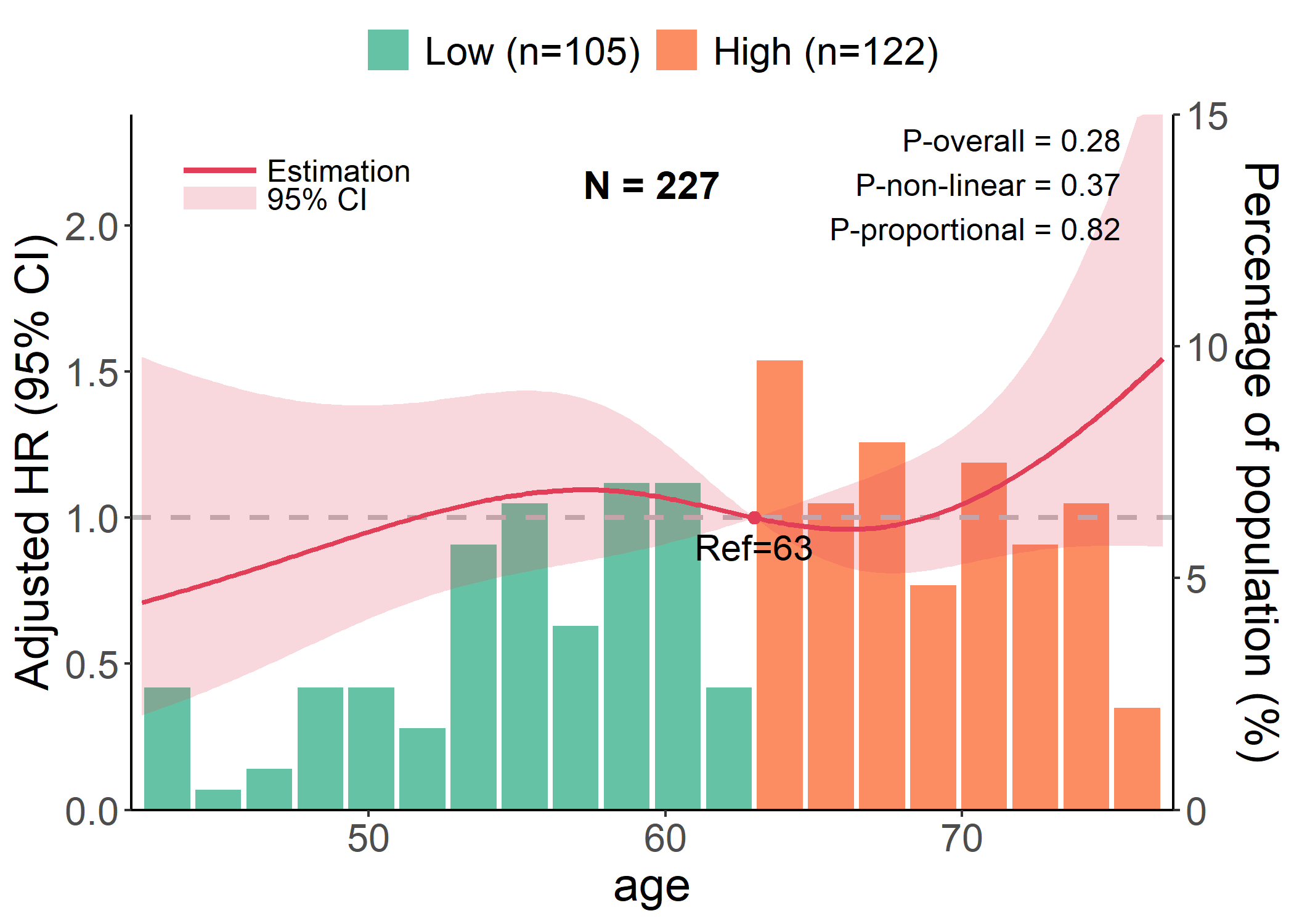
Example 3.3: RCS Plot
data(cancer, package = "survival")

# Performing cox regression, which is inferred by `y` and `time`
p <- rcs_plot(cancer, x = "age", y = "status", time = "time", covars = c("sex", "ph.karno"), save_plot = FALSE)
#> Warning in predictor_effect_plot(data = data, x = x, y = y, time = time, : 1
#> incomplete cases excluded.
plot(p)
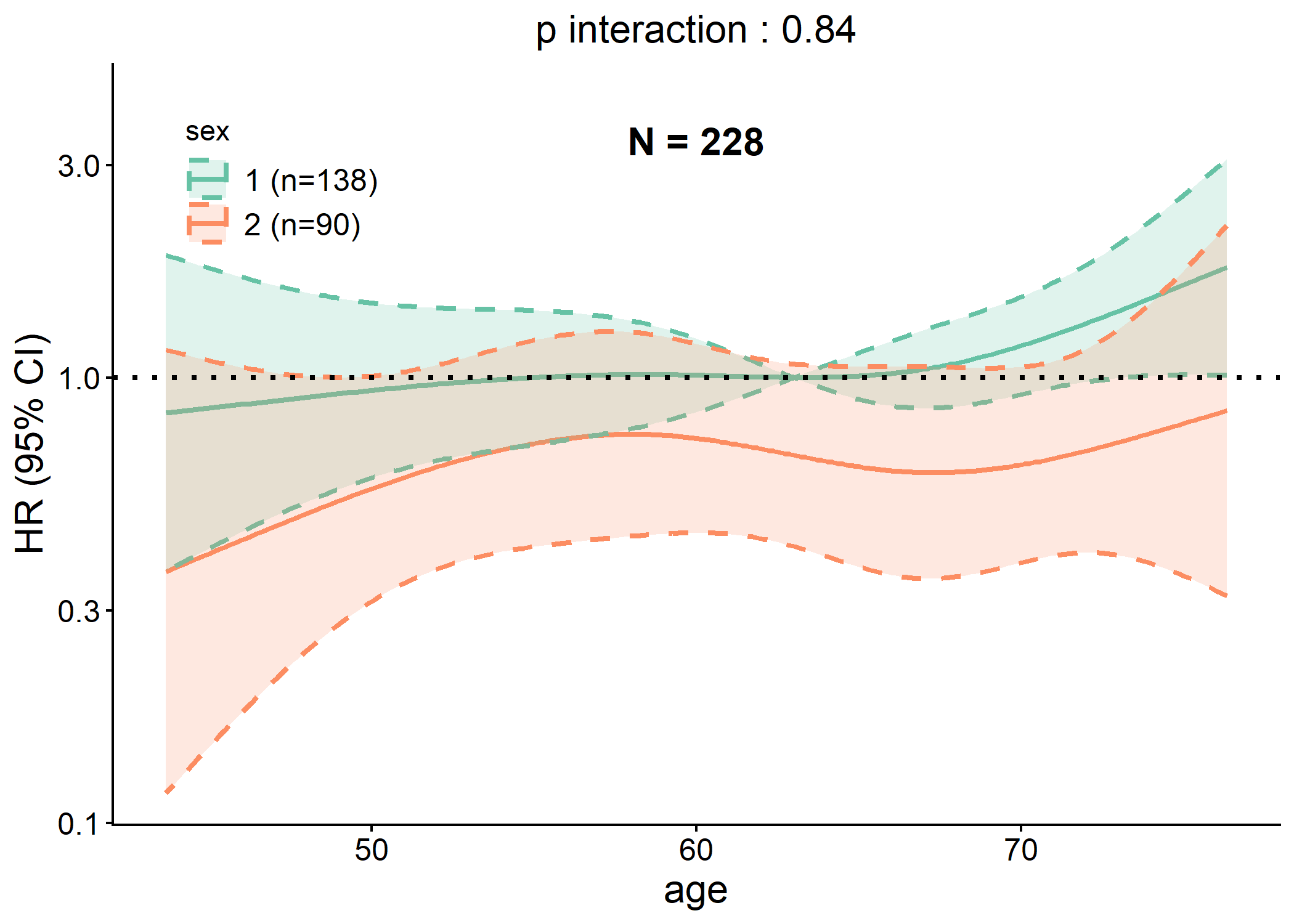
Example 3.4: Interaction Plot
data(cancer, package = "survival")

# Generating interaction plot of both linear and RCS models
p <- interaction_plot(cancer,
  y = "status", time = "time", predictor = "age",
  group_var = "sex", save_plot = FALSE
)
plot(p$lin)
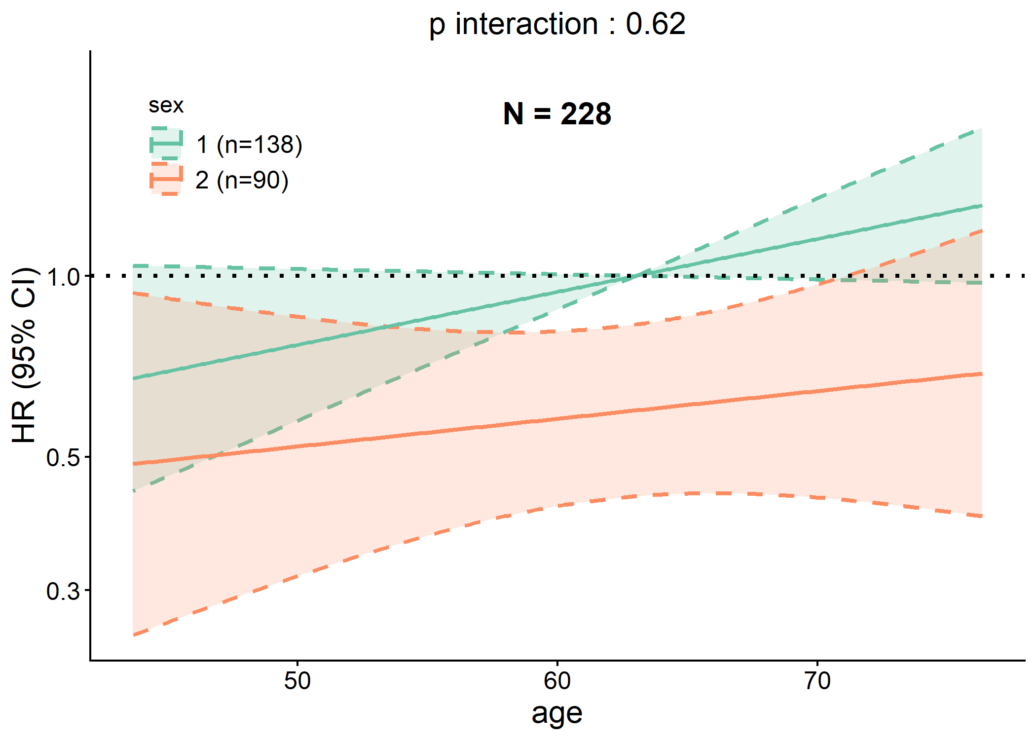
plot(p$rcs)
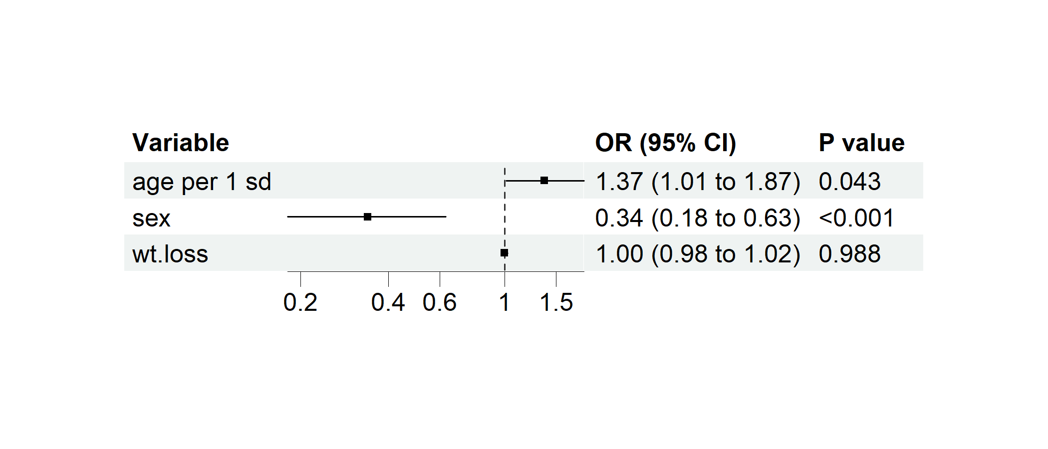
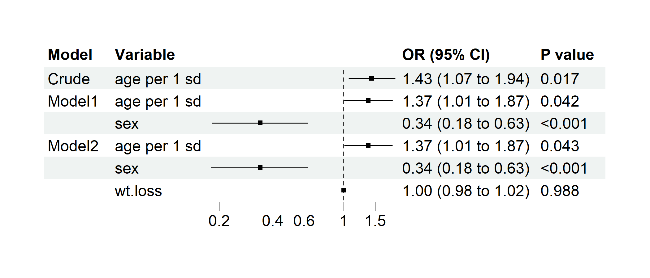
Example 3.5: Regression Forest Plot
data(cancer, package = "survival")
cancer$dead <- cancer$status == 2 # Preparing a binary variable for logistic regression
cancer$`age per 1 sd` <- c(scale(cancer$age)) # Standardizing age

# Performing multivairate logistic regression
p1 <- regression_forest(cancer,
  model_vars = c("age per 1 sd", "sex", "wt.loss"), y = "dead",
  as_univariate = FALSE, save_plot = FALSE
)
plot(p1)
p2 <- regression_forest(
  cancer,
  model_vars = list(
    Crude = c("age per 1 sd"),
    Model1 = c("age per 1 sd", "sex"),
    Model2 = c("age per 1 sd", "sex", "wt.loss")
  ),
  y = "dead",
  save_plot = FALSE
)
plot(p2)
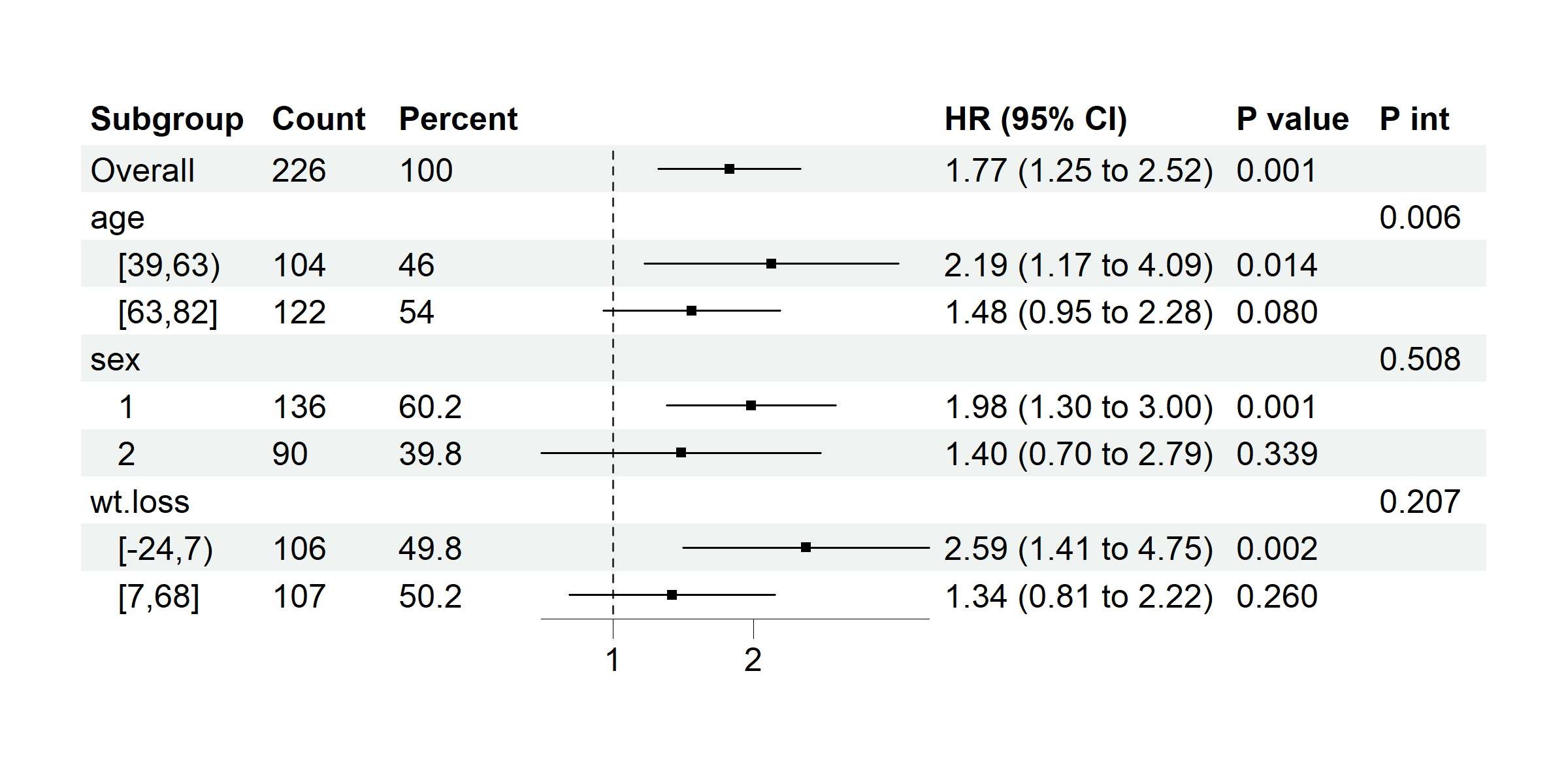
Example 3.6: Subgroup Forest Plot
data(cancer, package = "survival")
# coxph model with time assigned
p <- subgroup_forest(cancer,
  subgroup_vars = c("age", "sex", "wt.loss"), x = "ph.ecog", y = "status",
  time = "time", covars = "ph.karno", ticks_at = c(1, 2), save_plot = FALSE
)
plot(p)
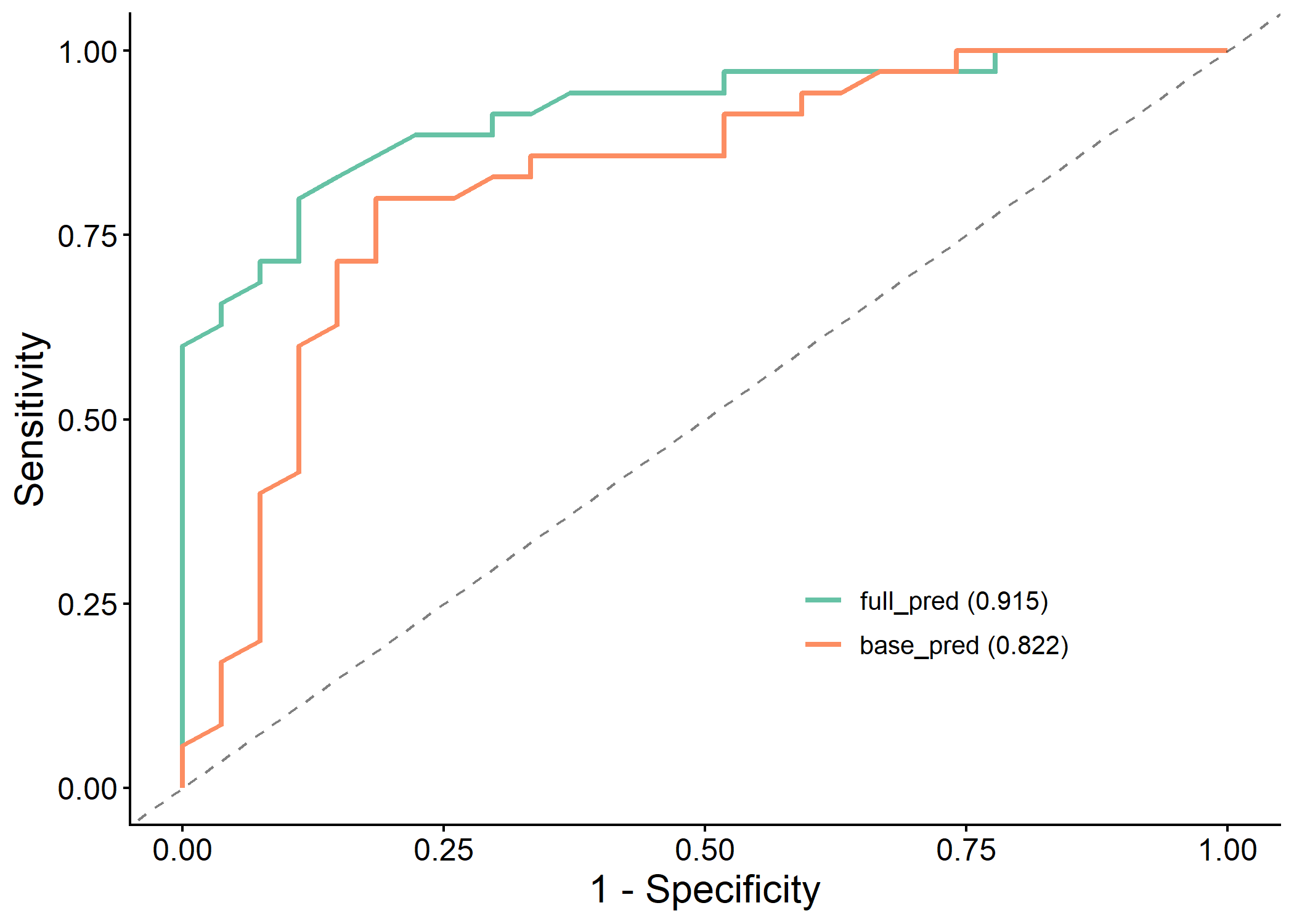
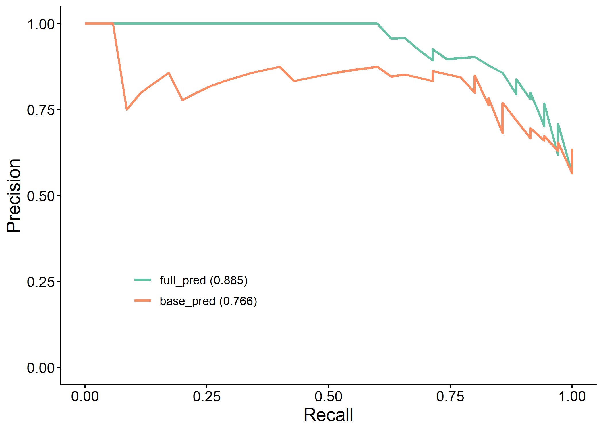
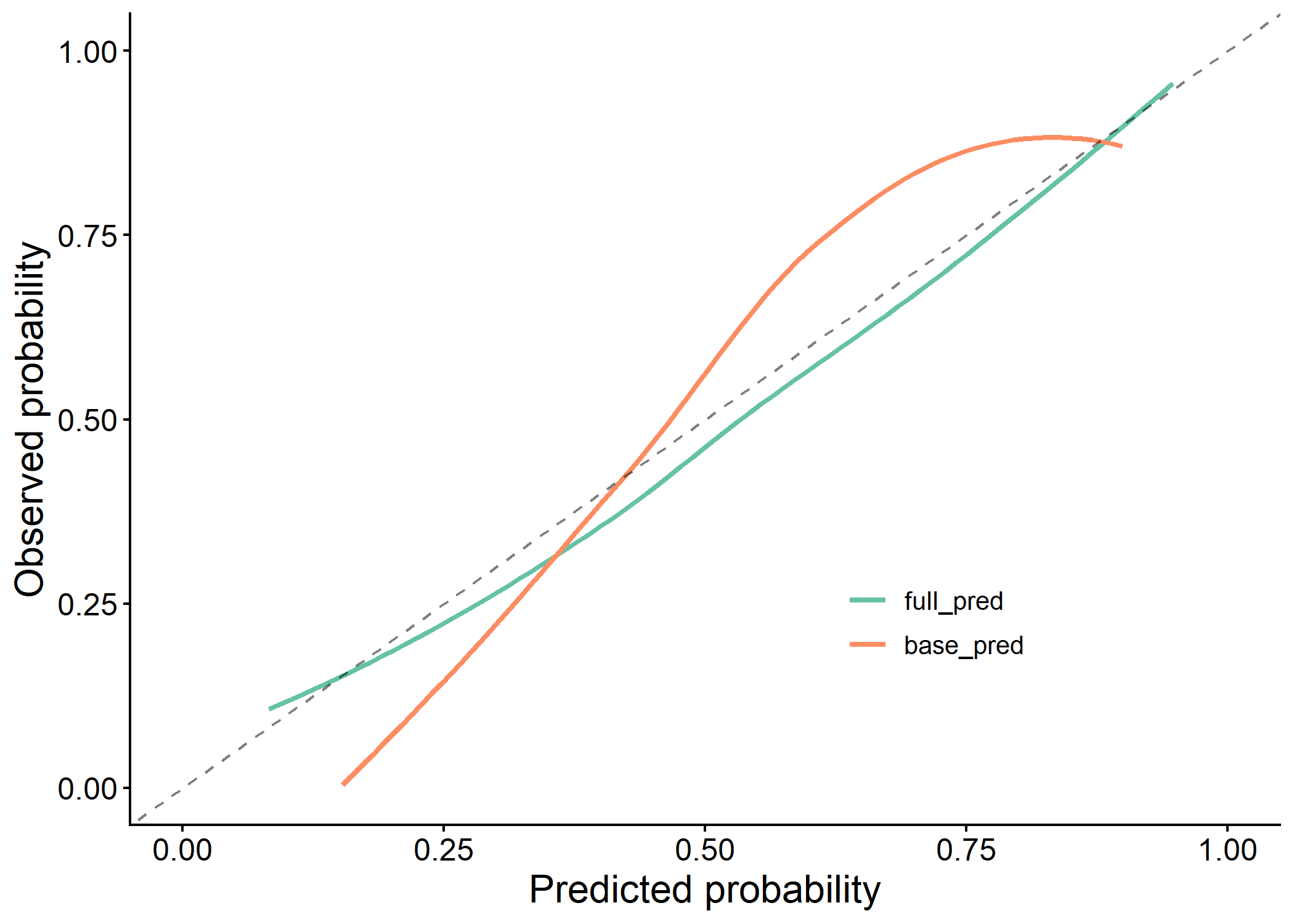
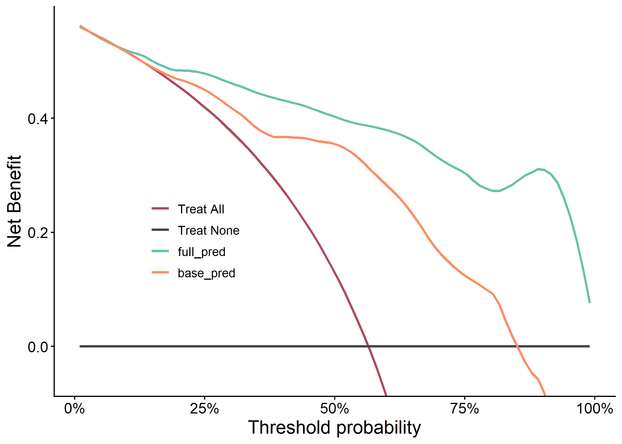
Example 3.7: Classification Model Performance
# Building models with example data
data(cancer, package = "survival")
df <- kidney
df$dead <- ifelse(df$time <= 100 & df$status == 0, NA, df$time <= 100)
df <- na.omit(df[, -c(1:3)])

model0 <- glm(dead ~ age + frail, family = binomial(), data = df)
model1 <- glm(dead ~ ., family = binomial(), data = df)
df$base_pred <- predict(model0, type = "response")
df$full_pred <- predict(model1, type = "response")

# Generating most of the useful plots and metrics for model comparison
results <- classif_model_compare(df, "dead", c("base_pred", "full_pred"), save_output = FALSE)
#> Assuming 'TRUE' is [Event] and 'FALSE' is [non-Event]

knitr::kable(results$metric_table)
| Model | AUC | PRAUC | Accuracy | Sensitivity | Specificity | Pos Pred Value | Neg Pred Value | F1 | Kappa | Brier | cutoff | Youden | HosLem | |
|---|---|---|---|---|---|---|---|---|---|---|---|---|---|---|
| 2 | full_pred | 0.915 (0.847, 0.984) | 0.885 | 0.839 | 0.8 | 0.889 | 0.903 | 0.774 | 0.848 | 0.677 | 0.114 | 0.626 | 0.689 | 0.944 |
| 1 | base_pred | 0.822 (0.711, 0.933) | 0.766 | 0.806 | 0.8 | 0.815 | 0.848 | 0.759 | 0.824 | 0.610 | 0.171 | 0.490 | 0.615 | 0.405 |
plot(results$roc_plot)
plot(results$pr_plot)
plot(results$calibration_plot)
plot(results$dca_plot)
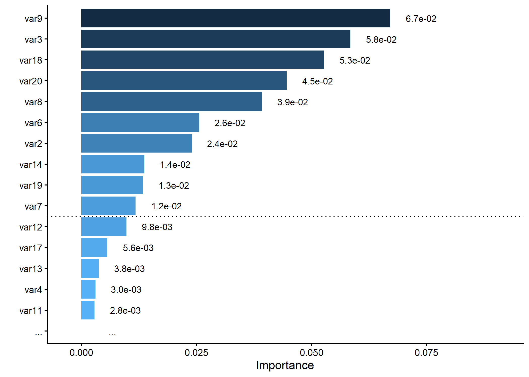
Example 3.8: Importance Plot
# Generating a dummy importance vector
set.seed(5)
dummy_importance <- runif(20, 0.2, 0.6)^5
names(dummy_importance) <- paste0("var", 1:20)

# Plotting variable importance, keeping only top 15 and splitting at 10
p <- importance_plot(dummy_importance, top_n = 15, split_at = 10, save_plot = FALSE)
plot(p)
#> Warning: Removed 1 row containing missing values or values outside the scale range
#> (`geom_bar()`).
Documentation
For detailed usage, refer to the package vignettes (coming soon) or the GitHub repository.
Contributing
Bug reports and feature requests are welcome via the issue tracker.
License
clinpubr is licensed under GPL (>= 3).