Assessing Predisposition Between Phenotypes using Polygenic Scores.
comorbidPGS

comorbidPGS is a tool for analysing an already computed Polygenic Score (PGS, also named PRS/GRS for binary outcomes) distribution to investigate shared genetic aetiology in multiple conditions.
comorbidPGS is under GPL-3 license, and is freely available for download.
Prerequisite
- R version 3.5 or higher with the following packages:
- stats
- utils
- ggplot2
Installation
comorbidPGS is available on CRAN, you can download it using the following command:
install.packages("comorbidPGS")
If you prefer the latest stable development version, you can download it from GitHub with:
if (!require("devtools", quietly = TRUE)) install.packages("devtools")
devtools::install_github("VP-biostat/comorbidPGS")
Example
Building an Association Table of PGS
This is a basic example which shows you how to do basic association with the example dataset:
library(comorbidPGS)
#>
#> Attaching package: 'comorbidPGS'
#> The following object is masked from 'package:graphics':
#>
#>     assocplot

# use the demo dataset
dataset <- comorbidData
# NOTE: The dataset must have at least 3 different columns:
# - an ID column (the first one)
# - a PGS column (must be numeric, by default it is the column named "SCORESUM" or the second column if "SCORESUM" is not present)
# - a Phenotype column, can be factors, numbers or characters

# do an association of one PGS with one Phenotype
result_1 <- assoc(dataset, prs_col = "t2d_PGS", phenotype_col = "t2d")
| PGS | Phenotype | Phenotype_type | Statistical_method | Covar | N_cases | N_controls | N | Effect | SE | lower_CI | upper_CI | P_value |
|---|---|---|---|---|---|---|---|---|---|---|---|---|
| t2d_PGS | t2d | Cases/Controls | Binary logistic regression | NA | 730 | 9270 | 10000 | 1.688258 | NA | 1.561821 | 1.824931 | 0 |
# do multiple associations
assoc <- expand.grid(c("t2d_PGS", "ldl_PGS"), c("ethnicity","brc","t2d","log_ldl","sbp_cat"))
result_2 <- multiassoc(df = dataset, assoc_table = assoc, covar = c("age", "sex", "gen_array"))
#> Warning in phenotype_type(df = df, phenotype_col = phenotype_col): Phenotype
#> column log_ldl is continuous and not normal, please normalise prior association

#> Warning in phenotype_type(df = df, phenotype_col = phenotype_col): Phenotype
#> column log_ldl is continuous and not normal, please normalise prior association
| PGS | Phenotype | Phenotype_type | Statistical_method | Covar | N_cases | N_controls | N | Effect | SE | lower_CI | upper_CI | P_value | |
|---|---|---|---|---|---|---|---|---|---|---|---|---|---|
| 2 | t2d_PGS | ethnicity 1 ~ 2 | Categorical | Multinomial logistic regression | age+sex+gen_array | 2142 | 6381 | 8523 | 0.9814174 | NA | 0.9345150 | 1.0306739 | 0.4528020 |
| 3 | t2d_PGS | ethnicity 1 ~ 3 | Categorical | Multinomial logistic regression | age+sex+gen_array | 1205 | 6381 | 7586 | 1.0178971 | NA | 0.9570931 | 1.0825640 | 0.5724292 |
| 4 | t2d_PGS | ethnicity 1 ~ 4 | Categorical | Multinomial logistic regression | age+sex+gen_array | 272 | 6381 | 6653 | 0.9434640 | NA | 0.8355980 | 1.0652542 | 0.3474694 |
| 21 | ldl_PGS | ethnicity 1 ~ 2 | Categorical | Multinomial logistic regression | age+sex+gen_array | 2142 | 6381 | 8523 | 0.9925623 | NA | 0.9451678 | 1.0423334 | 0.7648927 |
| 31 | ldl_PGS | ethnicity 1 ~ 3 | Categorical | Multinomial logistic regression | age+sex+gen_array | 1205 | 6381 | 7586 | 1.0083869 | NA | 0.9481215 | 1.0724830 | 0.7905175 |
| 41 | ldl_PGS | ethnicity 1 ~ 4 | Categorical | Multinomial logistic regression | age+sex+gen_array | 272 | 6381 | 6653 | 0.9760204 | NA | 0.8647226 | 1.1016433 | 0.6943783 |
| 1 | t2d_PGS | brc | Cases/Controls | Binary logistic regression | age+sex+gen_array | 402 | 5041 | 5443 | 1.0061678 | NA | 0.9087543 | 1.1140235 | 0.9057882 |
| 11 | ldl_PGS | brc | Cases/Controls | Binary logistic regression | age+sex+gen_array | 402 | 5041 | 5443 | 1.1037106 | NA | 0.9956370 | 1.2235153 | 0.0605407 |
| 12 | t2d_PGS | t2d | Cases/Controls | Binary logistic regression | age+sex+gen_array | 730 | 9270 | 10000 | 1.7359738 | NA | 1.6029867 | 1.8799938 | 0.0000000 |
| 13 | ldl_PGS | t2d | Cases/Controls | Binary logistic regression | age+sex+gen_array | 730 | 9270 | 10000 | 0.9823272 | NA | 0.9102411 | 1.0601223 | 0.6465580 |
| 14 | t2d_PGS | log_ldl | Continuous | Linear regression | age+sex+gen_array | NA | NA | 10000 | 0.0059961 | 0.0022747 | 0.0015378 | 0.0104544 | 0.0084010 |
| 15 | ldl_PGS | log_ldl | Continuous | Linear regression | age+sex+gen_array | NA | NA | 10000 | 0.0828545 | 0.0021183 | 0.0787027 | 0.0870064 | 0.0000000 |
| 16 | t2d_PGS | sbp_cat | Ordered Categorical | Ordinal logistic regression | age+sex+gen_array | NA | NA | 10000 | 1.0628744 | NA | 1.0236044 | 1.1036509 | 0.0015002 |
| 17 | ldl_PGS | sbp_cat | Ordered Categorical | Ordinal logistic regression | age+sex+gen_array | NA | NA | 10000 | 1.0078855 | NA | 0.9707330 | 1.0464598 | 0.6818849 |
Extension of association analysis: one-sample MR using the Wald Ratio and 2SLS methods
# MR using Wald ratio method
mr1 <- mr_ratio(df = dataset, prs_col = "ldl_PGS", exposure_col = "log_ldl", outcome_col = "sbp")
#> Warning in phenotype_type(df = df, phenotype_col = exposure_col): Phenotype
#> column log_ldl is continuous and not normal, please normalise prior association
#> Warning in phenotype_type(df = df, phenotype_col = outcome_col): Phenotype
#> column sbp is continuous and not normal, please normalise prior association
| PGS | Exposure | Outcome | Method | N_cases | N_controls | N | MR_estimate | SE | F_stat | |
|---|---|---|---|---|---|---|---|---|---|---|
| ldl_PGS | ldl_PGS | log_ldl | sbp | Ratio | NA | NA | 10000 | 0.0321099 | 2.387691 | 1449.37 |
# MR using 2-stage least square method (2SLS)
mr2 <- mr_2sls(df = dataset, prs_col = "ldl_PGS", exposure_col = "log_ldl", outcome_col = "sbp")
#> Warning in phenotype_type(df = df, phenotype_col = exposure_col): Phenotype
#> column log_ldl is continuous and not normal, please normalise prior association
#> Warning in phenotype_type(df = df, phenotype_col = outcome_col): Phenotype
#> column sbp is continuous and not normal, please normalise prior association
| PGS | Exposure | Outcome | Method | N_cases | N_controls | N | MR_estimate | SE | F_stat | |
|---|---|---|---|---|---|---|---|---|---|---|
| value | ldl_PGS | log_ldl | sbp | 2SLS | NA | NA | 10000 | 0.0321099 | 2.387532 | 1449.37 |
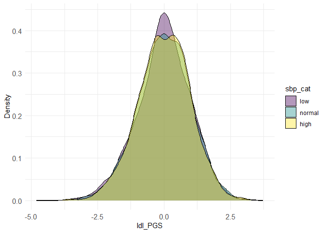
Examples of data visualisation using comorbidPGS
densityplot(dataset, prs_col = "ldl_PGS", phenotype_col = "sbp_cat")
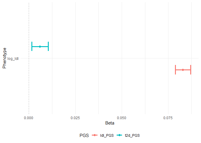
# show multiple associations in a plot
assoplot <- assocplot(score_table = result_2)
assoplot$continuous_phenotype
assoplot$discrete_phenotype
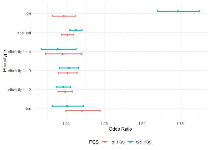 NOTE: The score_table should have the assoc() output format
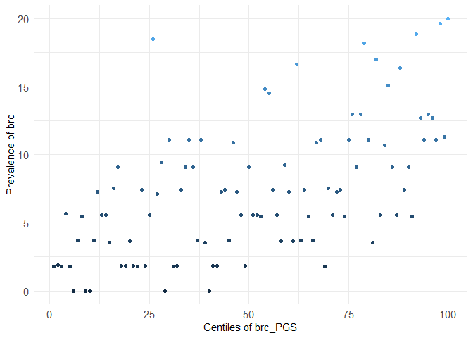
centileplot(dataset, prs_col = "brc_PGS", phenotype_col = "brc")
#> Warning in centileplot(dataset, prs_col = "brc_PGS", phenotype_col = "brc"):
#> The dataset has less than 10,000 individuals, centiles plot may not look good!
#> Use the argument decile = TRUE to adapt to small datasets
As those graphical functions use ggplot2, you can fully customize your plot:
library(ggplot2)
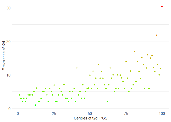
centileplot(dataset, prs_col = "t2d_PGS", phenotype_col = "t2d") +
scale_color_gradient(low = "green", high = "red")
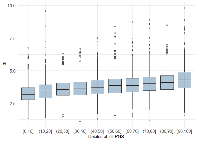
decileboxplot(dataset, prs_col = "ldl_PGS", phenotype_col = "ldl")
Citation
To cite comorbidPGS in publications, please use:
Pascat V, Zudina L, Ulrich A, Maina JG, Kaakinen M, Pupko I, Bonnefond A, Demirkan A, Balkhiyarova Z, Froguel P, Prokopenko I (2024). “comorbidPGS: an R package assessing shared predisposition between Phenotypes using Polygenic Scores.” Human Heredity. doi: 10.1159/000539325.