Description

Scientific Content and Citation Analysis from PDF Documents.

Description

Provides comprehensive tools for extracting and analyzing scientific content from PDF documents, including citation extraction, reference matching, text analysis, and bibliometric indicators. Supports multi-column PDF layouts, 'CrossRef' API <https://www.crossref.org/documentation/retrieve-metadata/rest-api/> integration, and advanced citation parsing.

README.md

cran.r-project.org

contentanalysis

Overview

contentanalysis is a comprehensive R package designed for in-depth analysis of scientific literature. It bridges the gap between raw PDF documents and structured, analyzable data by combining advanced text extraction, citation analysis, and bibliometric enrichment from external databases.

AI-Enhanced PDF Import: The package supports AI-assisted PDF text extraction through Google’s Gemini API, enabling more accurate parsing of complex document layouts. To use this feature, you need to obtain an API key from Google AI Studio.

Integration with bibliometrix: This package complements the science mapping analyses available in bibliometrix and its Shiny interface biblioshiny. If you want to perform content analysis within a user-friendly Shiny application with all the advantages of an interactive interface, simply install bibliometrix and launch biblioshiny, where you’ll find a dedicated Content Analysis menu that implements all the analyses and outputs of this library.

What Makes It Unique?

The package goes beyond simple PDF parsing by creating a multi-layered analytical framework:

Intelligent PDF Processing: Extracts text from multi-column PDFs while preserving document structure (sections, paragraphs, references)
Citation Intelligence: Detects and extracts citations in multiple formats (numbered, author-year, narrative, parenthetical) and maps them to their precise locations in the document
Bibliometric Enrichment: Automatically retrieves and integrates metadata from external sources:

CrossRef API: Retrieves structured reference data including authors, publication years, journals, and DOIs
OpenAlex: Enriches references with additional metadata, filling gaps and providing comprehensive bibliographic information

Citation-Reference Linking: Implements sophisticated matching algorithms to connect in-text citations with their corresponding references, handling various citation styles and ambiguous cases
Context-Aware Analysis: Extracts the textual context surrounding each citation, enabling semantic analysis of how references are used throughout the document
Network Visualization: Creates interactive networks showing citation co-occurrence patterns and conceptual relationships within the document

The Complete Workflow

PDF Document → Text Extraction → Citation Detection → Reference Parsing
↓
CrossRef/OpenAlex APIs
↓
Citation-Reference Matching → Enriched Dataset
↓
Network Analysis + Text Analytics + Bibliometric Indicators

The result is a rich, structured dataset that transforms a static PDF into an analyzable knowledge object, ready for: - Content analysis: Understanding what concepts and methods are discussed - Citation analysis: Examining how knowledge is constructed and referenced - Temporal analysis: Tracking the evolution of ideas through citation patterns - Network analysis: Visualizing intellectual connections - Readability assessment: Evaluating text complexity and accessibility

Key Features

PDF Import & Text Extraction

Multi-column layout support with automatic section detection
Structure preservation (title, abstract, introduction, methods, results, discussion, references)
Handling of complex layouts and special characters
DOI extraction from PDF metadata

Citation Extraction & Analysis

Comprehensive detection of citation formats:
- Numbered citations: [1], [1-3], [1,5,7]
Author-year citations: (Smith, 2020), (Smith et al., 2020)
Narrative citations: Smith (2020) demonstrated...
Complex citations: (see Smith, 2020; Jones et al., 2021)
Citation context extraction (surrounding text analysis)
Citation positioning and density metrics
Section-wise citation distribution

Reference Management & Enrichment

Local parsing: Extract references from the document’s reference section
CrossRef integration: Retrieve structured metadata for cited works via DOI
OpenAlex integration: Enrich references with additional bibliographic data
Automatic gap-filling: Complete missing author names, years, journal names
Structured reference format: Standardized author lists, publication years, journals

Citation-Reference Matching

Intelligent matching algorithms with multiple confidence levels:
- High confidence: Exact author-year matches
- Medium confidence: Fuzzy matching for variant author names
- Disambiguation: Handles multiple works by the same author
Support for various citation styles (APA, Chicago, Vancouver, etc.)
Handles complex cases: multiple authors, “et al.”, year suffixes (2020a, 2020b)

Network Analysis

Interactive citation co-occurrence networks
Distance-based edge weighting (closer citations = stronger connections)
Section-aware visualization (color-coded by document section)
Multi-section citation detection (citations appearing in multiple sections)
Network statistics: centrality, clustering, community detection potential
Citation cluster descriptions: TF-IDF analysis of reference titles by section
Interactive plotly visualizations: bar charts, heatmaps, and reference density plots

Text Analysis

Word frequency analysis with stopword removal
N-gram extraction (bigrams, trigrams)
Lexical diversity metrics
Readability indices (Flesch, Gunning Fog, SMOG, Coleman-Liau)
Word distribution tracking across document sections
Methodological term tracking

Bibliometric Indicators

Citation density (citations per 1000 words)
Citation type distribution (narrative vs. parenthetical)
Co-citation analysis
Reference age distribution
Journal diversity metrics

Installation

You can install the development version from GitHub:

# install.packages("devtools")
devtools::install_github("massimoaria/contentanalysis")

Example

Complete workflow analyzing a real scientific paper:

library(contentanalysis)

Download example paper

The paper is an open access article by Aria et al.:

Aria, M., Cuccurullo, C., & Gnasso, A. (2021). A comparison among interpretative proposals for Random Forests. Machine Learning with Applications, 6, 100094.

paper_url <- "https://raw.githubusercontent.com/massimoaria/contentanalysis/master/inst/examples/example_paper.pdf"
download.file(paper_url, destfile = "example_paper.pdf", mode = "wb")

Import PDF with automatic section detection

doc <- pdf2txt_auto("example_paper.pdf",
                    n_columns = 2,
                    citation_type = "author_year")
#> Stripped running header (6 occurrences, 40 chars)
#> Using 17 sections from PDF table of contents
#> Found 16 sections: Preface, Introduction, Related work, Internal processing approaches, Random forest extra information, Visualization toolkits, Post-Hoc approaches, Size reduction, Rule extraction, Local explanation, Comparison study, Experimental design, Analysis, Conclusion, Acknowledgment, References
#> Normalized 77 references with consistent \n\n separators

# Check detected sections
names(doc)
#>  [1] "Full_text"                       "Preface"                        
#>  [3] "Introduction"                    "Related work"                   
#>  [5] "Internal processing approaches"  "Random forest extra information"
#>  [7] "Visualization toolkits"          "Post-Hoc approaches"            
#>  [9] "Size reduction"                  "Rule extraction"                
#> [11] "Local explanation"               "Comparison study"               
#> [13] "Experimental design"             "Analysis"                       
#> [15] "Conclusion"                      "Acknowledgment"                 
#> [17] "References"

Perform comprehensive content analysis with CrossRef and OpenAlex enrichment

analysis <- analyze_scientific_content(
  text = doc,
  doi = "10.1016/j.mlwa.2021.100094",
  mailto = "[email protected]",
  citation_type = "author_year"
)
#> Extracting author-year citations only
#> Attempting to retrieve references from CrossRef...
#> Successfully retrieved 33 references from CrossRef
#> Fetching Open Access metadata for 14 DOIs from OpenAlex...
#> Successfully retrieved metadata for 13 references from OpenAlex

This single function call:

Extracts all citations from the document
Retrieves reference metadata from CrossRef using the paper’s DOI
Enriches references with additional data from OpenAlex
Matches citations to references with confidence scoring
Performs text analysis and computes bibliometric indicators

View summary statistics

analysis$summary
#> $total_words_analyzed
#> [1] 3453
#> 
#> $unique_words
#> [1] 1310
#> 
#> $citations_extracted
#> [1] 49
#> 
#> $narrative_citations
#> [1] 15
#> 
#> $parenthetical_citations
#> [1] 34
#> 
#> $complex_citations_parsed
#> [1] 12
#> 
#> $lexical_diversity
#> [1] 0.3793802
#> 
#> $average_citation_context_length
#> [1] 3230.429
#> 
#> $citation_density_per_1000_words
#> [1] 6.47
#> 
#> $references_parsed
#> [1] 33
#> 
#> $citations_matched_to_refs
#> [1] 42
#> 
#> $match_quality
#> # A tibble: 3 × 3
#>   match_confidence     n percentage
#>   <chr>            <int>      <dbl>
#> 1 high                42       85.7
#> 2 no_match_author      6       12.2
#> 3 no_match_year        1        2  
#> 
#> $citation_type_used
#> [1] "author_year"

Readability indices

readability <- calculate_readability_indices(doc$Full_text, detailed = TRUE)
readability
#> # A tibble: 1 × 12
#>   flesch_kincaid_grade flesch_reading_ease automated_readability_index
#>                  <dbl>               <dbl>                       <dbl>
#> 1                 12.7                33.3                        12.1
#> # ℹ 9 more variables: gunning_fog_index <dbl>, n_sentences <int>,
#> #   n_words <int>, n_syllables <dbl>, n_characters <int>,
#> #   n_complex_words <int>, avg_sentence_length <dbl>,
#> #   avg_syllables_per_word <dbl>, pct_complex_words <dbl>

Examine citations by type

analysis$citation_metrics$type_distribution
#> # A tibble: 11 × 3
#>    citation_type                   n percentage
#>    <chr>                       <int>      <dbl>
#>  1 parsed_from_multiple           12      24.5 
#>  2 author_year_basic               9      18.4 
#>  3 narrative_etal                  7      14.3 
#>  4 author_year_and                 6      12.2 
#>  5 author_year_etal                3       6.12
#>  6 narrative_three_authors_and     3       6.12
#>  7 narrative_two_authors_and       3       6.12
#>  8 narrative_four_authors_and      2       4.08
#>  9 see_citations                   2       4.08
#> 10 author_year_ampersand           1       2.04
#> 11 doi_pattern                     1       2.04

Analyze citation contexts

head(analysis$citation_contexts[, c("citation_text_clean", "section", "full_context")])
#> # A tibble: 6 × 3
#>   citation_text_clean                                       section full_context
#>   <chr>                                                     <chr>   <chr>       
#> 1 (Mitchell, 1997)                                          Introd… systems ide…
#> 2 https://doi.org/10.1016/j.mlwa.2021.100094                Introd… interpretat…
#> 3 (Breiman, 2001)                                           Introd… random subs…
#> 4 (see Breiman, 1996)                                       Introd… model that …
#> 5 (Hastie, supervised learning (Breiman, Friedman, Tibshir… Introd… by calculat…
#> 6 (Hastie et al., 2009)                                     Introd… but it is n…

Citation Network Visualization

Create interactive network visualizations showing how citations co-occur within your document:

# Create citation network
network <- create_citation_network(
  citation_analysis_results = analysis,
  max_distance = 800,          # Max distance between citations (characters)
  min_connections = 2,          # Minimum connections to include a node
  show_labels = TRUE
)

# Display interactive network
network

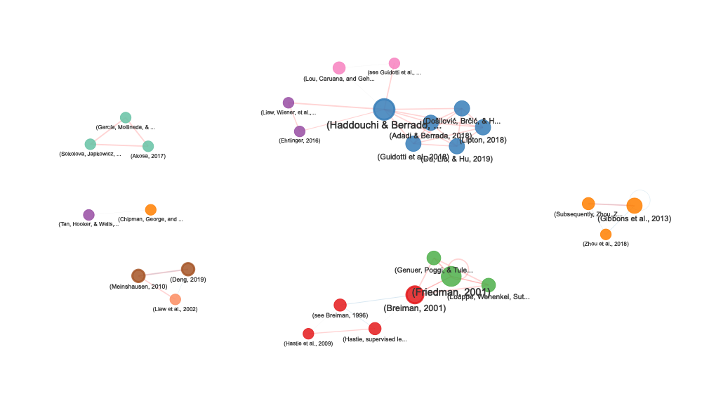
Access network statistics

stats <- attr(network, "stats")

# Network size
cat("Nodes:", stats$n_nodes, "\n")
#> Nodes: 28
cat("Edges:", stats$n_edges, "\n")
#> Edges: 49
cat("Average distance:", stats$avg_distance, "characters\n")
#> Average distance: 245.4 characters

# Citations by section
print(stats$section_distribution)
#>                   primary_section n
#> 1                    Related work 6
#> 2                    Introduction 4
#> 3                  Size reduction 4
#> 4             Experimental design 3
#> 5 Random forest extra information 3
#> 6          Visualization toolkits 3
#> 7               Local explanation 2
#> 8                 Rule extraction 2
#> 9                        Analysis 1

# Multi-section citations
if (nrow(stats$multi_section_citations) > 0) {
  print(stats$multi_section_citations)
}
#>                 citation_text
#> 1             (Breiman, 2001)
#> 2 (Haddouchi & Berrado, 2019)
#> 3         (Meinshausen, 2010)
#> 4                (Deng, 2019)
#>                                                         sections n_sections
#> 1                  Introduction, Random forest extra information          2
#> 2 Related work, Random forest extra information, Rule extraction          3
#> 3                    Rule extraction, Comparison study, Analysis          3
#> 4                    Rule extraction, Comparison study, Analysis          3

Network Features

The citation network visualization includes:

Node size: Proportional to number of connections
Node color: Indicates the primary section where citations appear
Node border: Thicker border (3px) for citations appearing in multiple sections
Edge thickness: Decreases with distance (closer citations = thicker edges)
Edge color:
- Red: Very close citations (≤300 characters)
Blue: Moderate distance (≤600 characters)
Gray: Distant citations (>600 characters)
Interactive features: Zoom, pan, drag nodes, highlight neighbors on hover

Customizing the Network

# Focus on very close citations only
network_close <- create_citation_network(
  analysis,
  max_distance = 300,
  min_connections = 1
)

# Show only highly connected citations
network_hubs <- create_citation_network(
  analysis,
  max_distance = 1000,
  min_connections = 5
)

# Hide labels for cleaner visualization
network_clean <- create_citation_network(
  analysis,
  show_labels = FALSE
)

Citation Cluster Description

Describe the thematic focus of each section’s bibliography using TF-IDF analysis of reference titles:

# Generate cluster descriptions
cluster_desc <- describe_citation_clusters(analysis, top_n = 10)

# View summary: top terms per section
cluster_desc$cluster_summary
#> # A tibble: 10 × 3
#>    section                         n_references top_terms                       
#>    <chr>                                  <int> <chr>                           
#>  1 Introduction                               4 learning, machine, machine lear…
#>  2 Related work                               8 black, black box, box, acm, sur…
#>  3 Random forest extra information            5 forests, random forests, annals…
#>  4 Visualization toolkits                     4 analytics, analytics ieee, comp…
#>  5 Size reduction                             4 adaptive, adaptive diagnostic, …
#>  6 Rule extraction                            2 annals applied, applied, applie…
#>  7 Local explanation                          3 models, classification, classif…
#>  8 Comparison study                           1 annals applied, applied, applie…
#>  9 Experimental design                        3 bell, bell laboratories, labora…
#> 10 Analysis                                   3 domains, domains acm, imbalance…

# View detailed TF-IDF scores
cluster_desc$cluster_descriptions
#> # A tibble: 83 × 7
#>    section      ngram              ngram_size     n     tf   idf tf_idf
#>    <chr>        <chr>                   <int> <int>  <dbl> <dbl>  <dbl>
#>  1 Introduction learning                    1     2 0.143   1.20 0.172 
#>  2 Introduction machine                     1     2 0.143   1.20 0.172 
#>  3 Introduction machine learning            2     2 0.143   1.20 0.172 
#>  4 Introduction bagging                     1     1 0.0714  2.30 0.164 
#>  5 Introduction bagging predictors          2     1 0.0714  2.30 0.164 
#>  6 Introduction predictors                  1     1 0.0714  2.30 0.164 
#>  7 Introduction predictors machine          2     1 0.0714  2.30 0.164 
#>  8 Introduction forests machine             2     1 0.0714  1.61 0.115 
#>  9 Introduction forests                     1     1 0.0714  1.20 0.0860
#> 10 Introduction random forests              2     1 0.0714  1.20 0.0860
#> # ℹ 73 more rows

Visualize Citation Clusters

Create interactive plotly visualizations that complement the citation network:

1. TF-IDF terms per section (2-column grid layout)

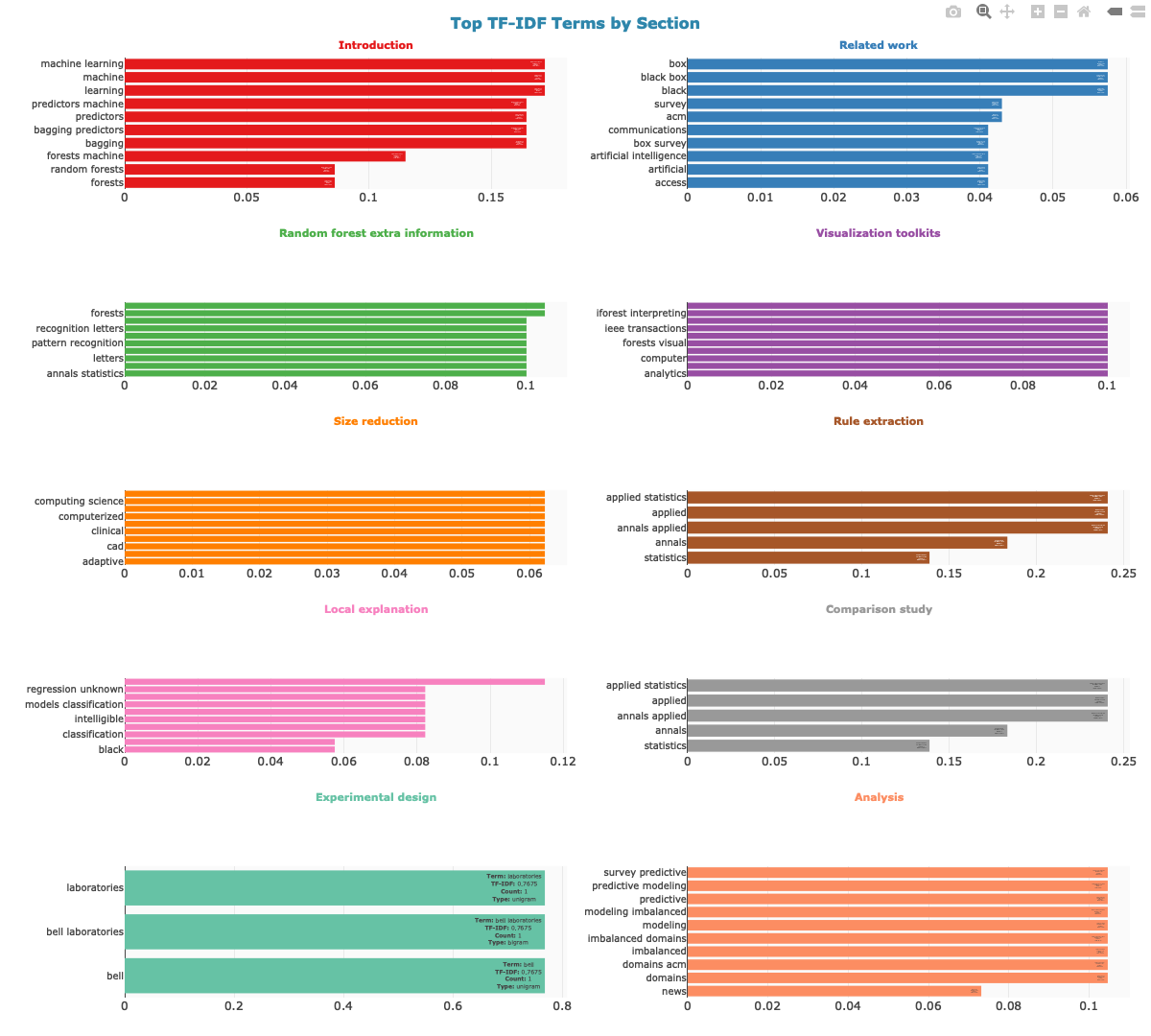
2. Heatmap: terms vs sections (unique vs shared terms)

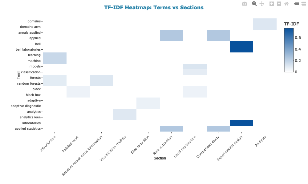
3. References per section

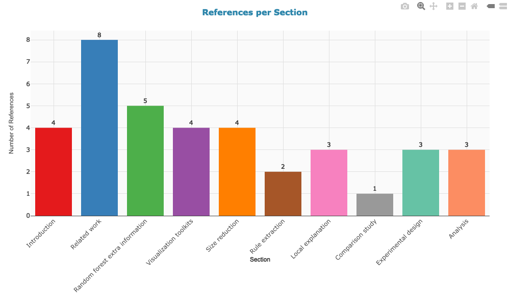
The TF-IDF bar chart uses a 2-column grid layout with color-coded section titles for a compact, readable overview. All plots display sections in the order they appear in the paper, use consistent styling, and include interactive hover information. Colors match the section colors used in the citation network.

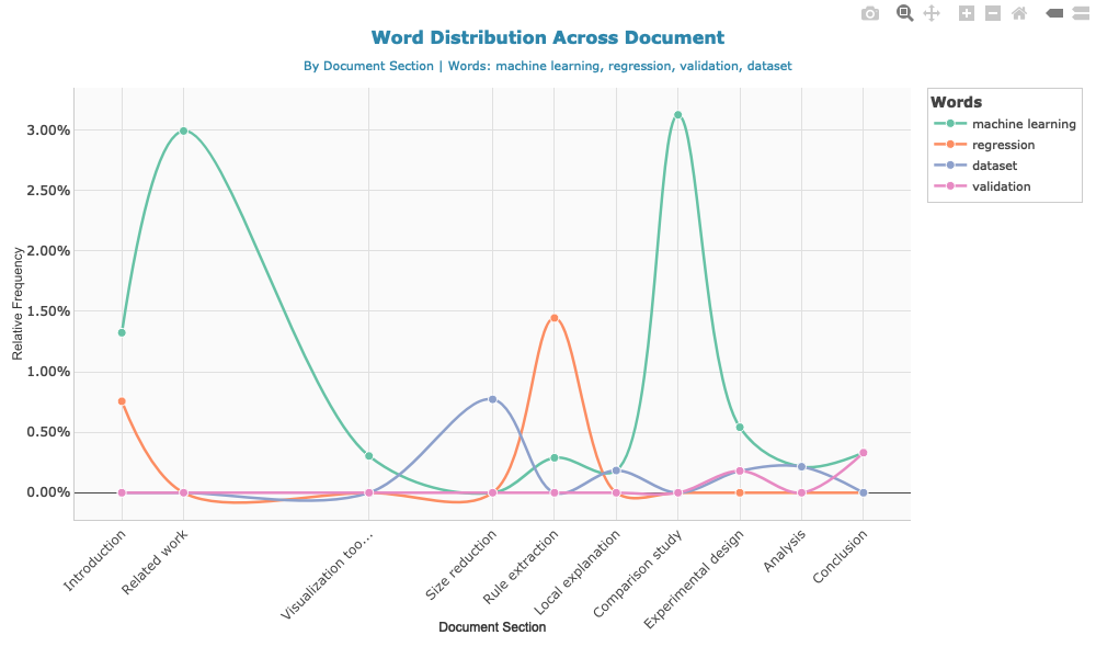
Text Analysis

Track methodological terms across sections

method_terms <- c("machine learning", "regression", "validation", "dataset")
word_dist <- calculate_word_distribution(doc, method_terms)

Create interactive visualization

Examine most frequent words

head(analysis$word_frequencies, 10)
#> # A tibble: 10 × 4
#>    word         n frequency  rank
#>    <chr>    <int>     <dbl> <int>
#>  1 model       45   0.0130      1
#>  2 forest      42   0.0122      2
#>  3 accuracy    40   0.0116      3
#>  4 trees       38   0.0110      4
#>  5 random      34   0.00985     5
#>  6 learning    27   0.00782     6
#>  7 set         27   0.00782     7
#>  8 variable    26   0.00753     8
#>  9 data        25   0.00724     9
#> 10 rule        25   0.00724    10

Citation co-occurrence data

head(analysis$network_data)
#> # A tibble: 6 × 5
#>   citation1                                       citation2 distance type1 type2
#>   <chr>                                           <chr>        <int> <chr> <chr>
#> 1 (Mitchell, 1997)                                https://…      734 auth… doi_…
#> 2 (Breiman, 2001)                                 (see Bre…      318 auth… see_…
#> 3 (Breiman, 2001)                                 (Hastie,…      734 auth… auth…
#> 4 (see Breiman, 1996)                             (Hastie,…      398 see_… auth…
#> 5 (see Breiman, 1996)                             (Hastie …      685 see_… auth…
#> 6 (Hastie, supervised learning (Breiman, Friedma… (Hastie …      210 auth… auth…

Working with References

Exploring enriched reference data

# View parsed references (enriched with CrossRef and OpenAlex)
head(analysis$parsed_references[, c("ref_first_author", "ref_year", "ref_journal", "ref_source")])
#>   ref_first_author ref_year           ref_journal ref_source
#> 1            Adadi     2018           IEEE Access   crossref
#> 2             <NA>     <NA>                  <NA>   crossref
#> 3           Branco     2016 ACM Computing Surveys   crossref
#> 4          Breiman     1996      Machine Learning   crossref
#> 5          Breiman     2001      Machine Learning   crossref
#> 6          Breiman     1984   International Group   crossref

# Check data sources
table(analysis$parsed_references$ref_source)
#> 
#> crossref 
#>       33

The ref_source column indicates where the data came from:

"crossref": Retrieved from CrossRef API
"parsed": Extracted from document’s reference section
References may be enriched with OpenAlex data even if originally from CrossRef

Analyzing citation-reference links

# View citation-reference matches with confidence levels
library(dplyr)
#> 
#> Attaching package: 'dplyr'
#> The following objects are masked from 'package:stats':
#> 
#>     filter, lag
#> The following objects are masked from 'package:base':
#> 
#>     intersect, setdiff, setequal, union
head(analysis$citation_references_mapping[, c("citation_text_clean", "ref_authors",
                                               "ref_year", "match_confidence")])
#> # A tibble: 6 × 4
#>   citation_text_clean                      ref_authors ref_year match_confidence
#>   <chr>                                    <chr>       <chr>    <chr>           
#> 1 (Mitchell, 1997)                         Mitchell    1997     high            
#> 2 https://doi.org/10.1016/j.mlwa.2021.100… <NA>        <NA>     no_match_year   
#> 3 (Breiman, 2001)                          Breiman, L. 2001     high            
#> 4 (see Breiman, 1996)                      Breiman, L. 1996     high            
#> 5 (Hastie, supervised learning (Breiman, … Hastie      2009     high            
#> 6 (Hastie et al., 2009)                    Hastie      2009     high

# Match quality distribution
table(analysis$citation_references_mapping$match_confidence)
#> 
#>            high no_match_author   no_match_year 
#>              42               6               1

Finding citations to specific authors

# Find all citations to works by Smith
analysis$citation_references_mapping %>%
  filter(grepl("Smith", ref_authors, ignore.case = TRUE)) %>%
  select(citation_text_clean, ref_full_text, match_confidence)
#> # A tibble: 0 × 3
#> # ℹ 3 variables: citation_text_clean <chr>, ref_full_text <chr>,
#> #   match_confidence <chr>

Accessing OpenAlex metadata

# If OpenAlex data was retrieved
if (!is.null(analysis$references_oa)) {
  # View enriched metadata
  head(analysis$references_oa[, c("title", "publication_year", "cited_by_count",
                                   "type", "oa_status")])

  # Analyze citation impact
  summary(analysis$references_oa$cited_by_count)
}
#>    Min. 1st Qu.  Median    Mean 3rd Qu.    Max. 
#>     100     205    1056   12429    5399  119748

Citations by section

analysis$citation_metrics$section_distribution
#> # A tibble: 15 × 3
#>    section                             n percentage
#>    <fct>                           <int>      <dbl>
#>  1 Preface                             0       0   
#>  2 Introduction                        6      12.2 
#>  3 Related work                        9      18.4 
#>  4 Internal processing approaches      0       0   
#>  5 Random forest extra information     6      12.2 
#>  6 Visualization toolkits              4       8.16
#>  7 Post-Hoc approaches                 0       0   
#>  8 Size reduction                      6      12.2 
#>  9 Rule extraction                     3       6.12
#> 10 Local explanation                   5      10.2 
#> 11 Comparison study                    2       4.08
#> 12 Experimental design                 4       8.16
#> 13 Analysis                            4       8.16
#> 14 Conclusion                          0       0   
#> 15 Acknowledgment                      0       0

Advanced: Word Distribution Analysis

# Track disease-related terms
disease_terms <- c("covid", "pandemic", "health", "policy", "vaccination")
dist <- calculate_word_distribution(doc, disease_terms, use_sections = TRUE)

# View frequencies by section
dist %>%
  select(segment_name, word, count, percentage) %>%
  arrange(segment_name, desc(percentage))
#> # A tibble: 1 × 4
#>   segment_name word   count percentage
#>   <chr>        <chr>  <int>      <dbl>
#> 1 Conclusion   health     1      0.331

# Visualize trends
#plot_word_distribution(dist, plot_type = "area", smooth = FALSE)

Main Functions

PDF Import

pdf2txt_auto(): Import PDF with automatic section detection
reconstruct_text_structured(): Advanced text reconstruction
extract_doi_from_pdf(): Extract DOI from PDF metadata

Content Analysis

analyze_scientific_content(): Comprehensive content and citation analysis with API enrichment
parse_references_section(): Parse reference list from text
match_citations_to_references(): Match citations to references with confidence scoring
get_crossref_references(): Retrieve references from CrossRef API

Network Analysis

create_citation_network(): Create interactive citation co-occurrence network
describe_citation_clusters(): Describe citation clusters by section using TF-IDF on reference titles
plot_citation_clusters(): Create interactive plotly visualizations of citation cluster descriptions (TF-IDF bars, heatmap, references per section)

Text Analysis

calculate_readability_indices(): Compute readability scores (Flesch, Gunning Fog, SMOG, Coleman-Liau)
calculate_word_distribution(): Track word frequencies across document sections
readability_multiple(): Batch readability analysis for multiple documents

Visualization

plot_word_distribution(): Interactive visualization of word distribution across sections
plot_citation_clusters(): Interactive TF-IDF bar charts, heatmaps, and reference density plots

Utilities

get_example_paper(): Download example paper for testing
map_citations_to_segments(): Map citations to document sections/segments

External Data Sources

CrossRef API

The package integrates with CrossRef’s REST API to retrieve structured bibliographic data:

Endpoint: https://api.crossref.org/works/{doi}/references
Data retrieved: Authors, publication year, journal/source, article title, DOI
Rate limits: Polite pool requires email (use mailto parameter)
More info: https://api.crossref.org

OpenAlex API

OpenAlex provides comprehensive scholarly metadata:

Endpoint: Via openalexR package
Data retrieved: Complete author lists, citation counts, open access status, institutional affiliations
Rate limits: 100,000 requests/day (polite pool with email), 10 requests/second
API key: Optional, increases rate limits. Set with openalexR::oa_apikey()
More info: https://openalex.org

Setting Up API Access

Email for polite pool (recommended)

Both CrossRef and OpenAlex offer a polite pool for users who provide an email address. This gives you faster and more reliable access compared to anonymous requests. Simply pass your email via the mailto parameter:

analysis <- analyze_scientific_content(
  text = doc,
  doi = "10.xxxx/xxxxx",
  mailto = "[email protected]"  # Your email for polite pool access
)

The mailto parameter is used by both CrossRef and OpenAlex to route your requests through their polite pool, which provides higher rate limits and priority access.

OpenAlex API key (optional, for extended use)

For heavier usage, OpenAlex offers a free API key that further increases rate limits (from 10 to 100 requests/second). This is recommended if you plan to analyze many documents in batch.

Get your free API key at: https://openalex.org/users
Set it in your R session before running the analysis:

openalexR::oa_apikey("your-api-key-here")

You can also add this to your .Rprofile so it’s automatically set at startup:

# Add to ~/.Rprofile
openalexR::oa_apikey("your-api-key-here")

Dependencies

Core: pdftools, dplyr, tidyr, stringr, tidytext, tibble, httr2, visNetwork, openalexR

Suggested: plotly, RColorBrewer, scales (for visualization)

Citation

If you use this package in your research, please cite:

Massimo Aria & Corrado Cuccurullo (2025). contentanalysis: Scientific Content and Citation Analysis from PDF Documents.
R package version 0.2.0.
https://doi.org/10.32614/CRAN.package.contentanalysis

License

GPL (>= 3)

Issues and Contributions

Please report issues at: https://github.com/massimoaria/contentanalysis/issues

Contributions are welcome! Please feel free to submit a Pull Request.

contentanalysis

Overview

What Makes It Unique?

The Complete Workflow

Key Features

PDF Import & Text Extraction

Citation Extraction & Analysis

Reference Management & Enrichment

Citation-Reference Matching

Network Analysis

Text Analysis

Bibliometric Indicators

Installation

Example

Download example paper

Import PDF with automatic section detection

Perform comprehensive content analysis with CrossRef and OpenAlex enrichment

View summary statistics

Readability indices

Examine citations by type

Analyze citation contexts

Citation Network Visualization

Access network statistics

Network Features

Customizing the Network

Citation Cluster Description

Visualize Citation Clusters

Text Analysis

Track methodological terms across sections

Create interactive visualization

Examine most frequent words

Citation co-occurrence data

Working with References

Exploring enriched reference data

Analyzing citation-reference links

Finding citations to specific authors

Accessing OpenAlex metadata

Citations by section

Advanced: Word Distribution Analysis

Main Functions

PDF Import

Content Analysis

Network Analysis

Text Analysis

Visualization

Utilities

External Data Sources

CrossRef API

OpenAlex API

Setting Up API Access

Email for polite pool (recommended)

OpenAlex API key (optional, for extended use)

Dependencies

Citation

License

Issues and Contributions

Version

License

Status

Source

Homepage

Platforms78 (78)

Platforms (78)