Covariate Dependent Graph Estimation.

covdepGE

The conditional dependence structure (CDS) of a data matrix with $p$ variables can be modeled as an undirected graph with $p$ vertices, where two variables are connected if, and only if, the two variables are dependent given the remaining variables in the data. Gaussian graphical modeling (GGM) seeks to capture the CDS of the data under the assumption that the data are normally distributed. This distributional assumption is convenient for inference, as the CDS is given by the sparsity structure of the precision matrix, where the precision matrix is defined as the inverse covariance matrix of the data.

There is extensive GGM literature and many R packages for GGM, however, all make the restrictive assumption that the precision matrix is homogeneous throughout the data, or that there exists a partition of homogeneous subgroups. covdepGE avoids this strong assumption by utilizing information sharing to model the CDS as varying continuously with an extraneous covariate. Intuitively, this implies that observations having similar extraneous covariate values will have similar precision matrices.

To facilitate information sharing while managing complexity, covdepGE uses an efficient variational approximation conducted under the novel weighted pseudo-likelihood framework proposed by (1). covdepGE further accelerates inference by employing parallelism and executing expensive iterative computations in C++. Additionally, covdepGE offers a principled, data-driven approach for hyperparameter specification that only requires the user to input data and extraneous covariates to perform inference. Finally, covdepGE offers several wrappers around ggplot2 for seamless visualization of resulting estimates, such as matViz, inclusionCurve, and the S3 method plot.covdepGE.

Installation

You can install the released version of covdepGE from CRAN with:

install.packages("covdepGE")

And the development version from GitHub with:

# install.packages("devtools")
devtools::install_github("JacobHelwig/covdepGE")

Contributing

If you have an idea to improve covdepGE, considering forking the repo and creating a pull request or opening an issue.

Example

library(covdepGE)
library(ggplot2)

# get the data
set.seed(12)
data <- generateData()
X <- data$X
Z <- data$Z
interval <- data$interval
prec <- data$true_precision

# get overall and within interval sample sizes
p <- ncol(X)
n <- nrow(X)
n1 <- sum(interval == 1)
n2 <- sum(interval == 2)
n3 <- sum(interval == 3)

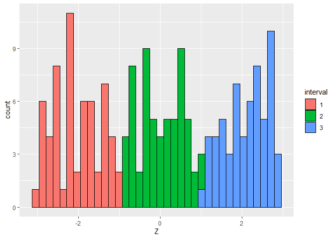
# visualize the distribution of the extraneous covariate
ggplot(data.frame(Z = Z, interval = as.factor(interval))) +
  geom_histogram(aes(Z, fill = interval), color = "black", bins = n %/% 5)

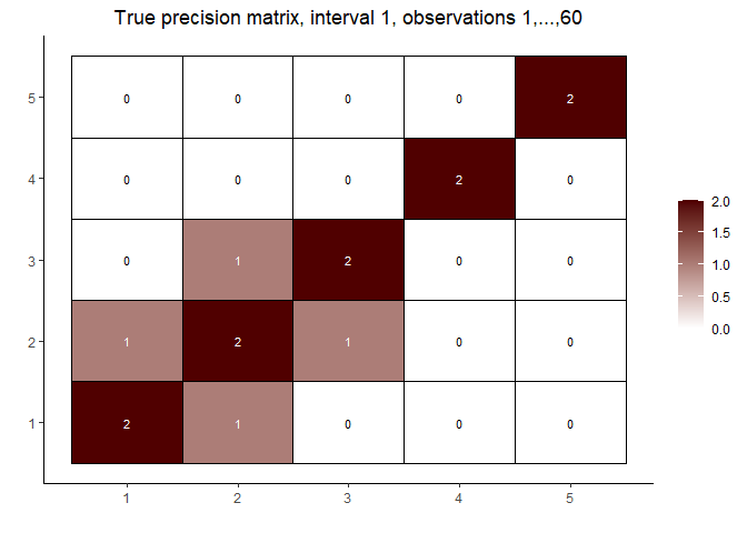
# visualize the true precision matrices in each of the intervals

# interval 1
matViz(prec[[1]], incl_val = TRUE) +
  ggtitle(paste0("True precision matrix, interval 1, observations 1,...,", n1))

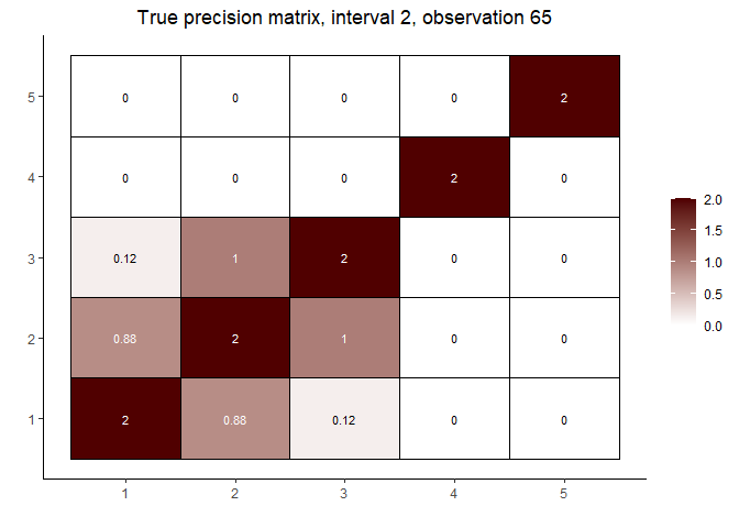
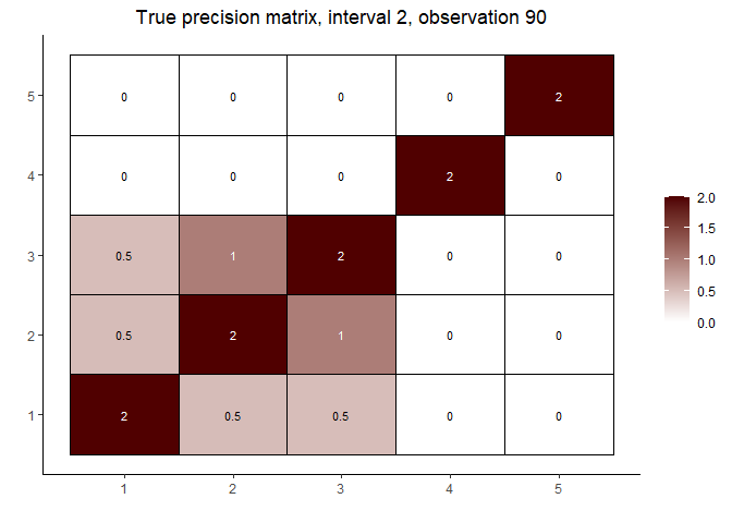
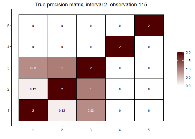
# interval 2 (varies continuously with Z)
cat("\nInterval 2, observations ", n1 + 1, ",...,", n1 + n2, sep = "")
#> 
#> Interval 2, observations 61,...,120
int2_mats <- prec[interval == 2]
int2_inds <- c(5, n2 %/% 2, n2 - 5)
lapply(int2_inds, function(j) matViz(int2_mats[[j]], incl_val = TRUE) +
         ggtitle(paste("True precision matrix, interval 2, observation", j + n1)))
#> [[1]]

#> 
#> [[2]]

#> 
#> [[3]]

# interval 3
matViz(prec[[length(prec)]], incl_val = TRUE) +
  ggtitle(paste0("True precision matrix, interval 3, observations ",
                 n1 + n2 + 1, ",...,", n1 + n2 + n3))

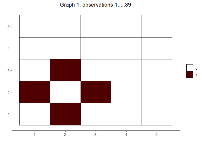
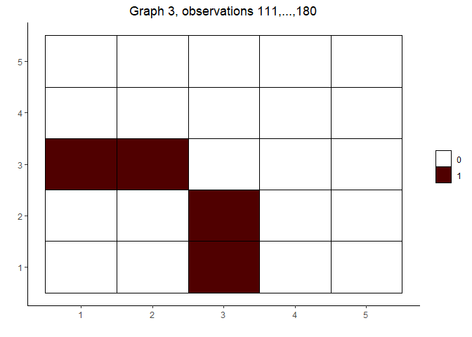
# fit the model and visualize the estimated graphs
(out <- covdepGE(X, Z, parallel = T, num_workers = p))
#> Warning in covdepGE(X, Z, parallel = T, num_workers = p): No registered workers
#> detected; registering doParallel with 5 workers
#>                       Covariate Dependent Graphical Model
#> 
#> ELBO: -171501.68                                             # Unique Graphs: 3
#> n: 180, variables: 5                       Hyperparameter grid size: 125 points
#> Model fit completed in 2.229 secs
plot(out)
#> [[1]]

#> 
#> [[2]]

#> 
#> [[3]]

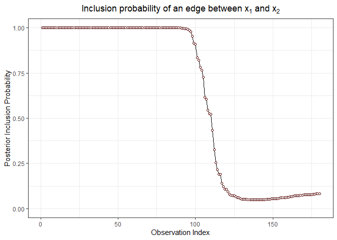
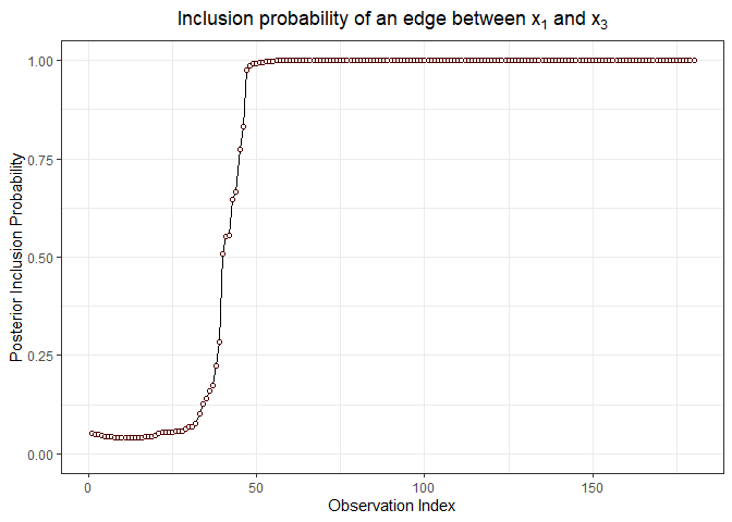
# visualize the posterior inclusion probabilities for variables (1, 3) and (1, 2)
inclusionCurve(out, 1, 2)

inclusionCurve(out, 1, 3)

Methods

Math is correctly rendered in the version of this document available on CRAN.

Overview

Suppose that $X$ is a $p$-dimensional data matrix with $n$ observations and that $Z$ is a $q$-dimensional extraneous covariate, also with $n$ observations, where the $l$-th observation in $Z$ is associated with the $l$-th observation in $X$. Further suppose that the $l$-th row of $X$ follows a $p$-dimensional Gaussian distribution with mean $0$ and precision matrix $\Omega(z_l)$, where $z_l$ is the $l$-th entry of $Z$ and $\Omega$ is a continuous function mapping from the space of extraneous covariates to the space of $p \times p$ non-singular matrices. Then, for the $l$-th observation, the $(j,k)$ entry of $\Omega(z_l)$ is non-zero if, and only if, variable $j$ and variable $k$ are dependent given the remaining variables in $X$.

Given data satisfying these assumptions, the covdepGE function employs the algorithm described in (1) to estimate a graphical representation of the structure of $\Omega$ for each of the observations in $X$ as a continuous function of $Z$. This graph contains an undirected edge between two variables $X_j$ and $X_k$ if, and only if, $X_j$ and $X_k$ are conditionally dependent given the remaining variables. Core components of this methodology are the weighted pseudo-likelihood framework in which inference is conducted via a block mean-field variational approximation.

Graph Estimation

Graphs are constructed using a pseudo-likelihood approach by fixing each of the columns $X_j$ of $X$ as the response and performing a spike-and-slab regression using the remaining variables $X_k$ in $X$ as predictors. To determine if an edge should be added between $X_j$ and $X_k$, the posterior inclusion probability of $X_k$ in a regression with $X_j$ fixed as the response ($PIP_j(X_k)$) and vice versa ($PIP_k(X_j)$) are symmetrized according to sym_method (e.g., by taking the mean of $PIP_k(X_j)$ and $PIP_j(X_k)$). If the symmetrized $PIP$ is greater than edge_threshold, an edge will be included between $X_j$ and $X_k$.

To model $\Omega$ as a function of $Z$, $n$ weighted spike-and-slab regressions are performed for each variable $X_j$ fixed as the response. The similarity weights for the $l$-th regression are taken with respect to observation $l$ such that observations having similar values of $Z$ will have larger weights. These similarity weights in conjunction with the pseudo-likelihood framework comprise the weighted pseudo-likelihood approach introduced by (1). Note that model performance is best when $n > p$.

Variational Inference

Spike-and-slab posterior quantities are estimated using a block mean-field variational approximation. Coordinate Ascent Variational Inference (CAVI) is performed for each of the weighted regressions to select the variational parameters that maximize the ELBO. The parameters for each of the regression coefficients are the mean and variance of the slab ($\mu$ and $\sigma^2_{\text{var}}$, respectively) and the probability that the coefficient is non-zero ($\alpha$). $\mu$ and $\alpha$ for all coefficients are initialized as $0$ and $0.2$, respectively.

CAVI for the $n$ regressions is performed simultaneously for variable $X_j$ fixed as the response. With each of the $n$ sets of $\alpha$ as the rows of an $n \times (p - 1)$ matrix, the CAVI for variable $X_j$ is ended for all $n$ regressions when the Frobenius norm of the change in the $\alpha$ matrix is less than alpha_tol or after max_iter iterations of CAVI have been performed.

Note that since the regressions performed for variable $X_j$ and $X_k$ fixed as the response are independent of each other, they may be performed in parallel by setting parallel = T. Registering parallel backend with greater than $p$ workers offers no benefit, since each worker takes on one variable to fix as the response and perform the $n$ regressions.

Hyperparameter specification

Each regression requires the specification of $3$ hyperparameters: $\pi$ (the prior probability of inclusion), $\sigma^2$ (the prior residual variance), and $\sigma_\beta^2$ (the prior variance of the slab). covdepGE offers $3$ methods for hyperparameter specification via the hp_method argument: grid_search, model_average, and hybrid. Empirically, grid_search offers the best sensitivity and model_average offers the best specificity, while hybrid sits between the other two methods in both metrics.

The hyperparameter candidate grid is generated by taking the Cartesian product between ssq, sbsq, and pip (candidate values for $\sigma^2$, $\sigma_\beta^2$, and $\pi$, respectively). Each of the methods gives an approach for selecting points from this grid.

In grid_search, the point from the grid that produces the model that has the greatest total ELBO is selected, where the total ELBO is calculated by summing the ELBO for each of the $n$ regressions for a variable $X_j$ fixed as the response. Thus, all observations use the same set of hyperparameters for the regression on $X_j$.

Instead of selecting only one model as in grid_search, models are averaged over in model_average. With $X_j$ fixed as the response, the unnormalized weights for each grid point used to perform this averaging is calculated by exponentiating the ELBO for each of the $n$ regressions. Note that since the ELBO for a given grid point will vary across the $n$ regressions due to differing similarity weights, each of the $n$ sets of averaging weights will be unique.

Finally, hybrid combines grid_search and model_average. Fixing $X_j$ as the response, for each $\pi$ candidate in pip, the point in the grid defined by the Cartesian product of ssq and sbsq is selected by maximizing the total ELBO summed across the $n$ regressions. The resulting models for each of the $\pi$ candidates are then averaged using the exponentiated ELBO for each of the $n$ regressions as the unnormalized averaging weights.

Note that in the search step of grid_search and hybrid, CAVI for each of the grid points is performed for at most max_iter_grid iterations. A second CAVI is then performed for max_iter iterations using the $n$ models that maximized the total ELBO in the first step. Setting max_iter_grid to be less than max_iter (as is the default) will result in a more efficient search.

Candidate grid generation

The candidate grids (ssq, sbsq, and pip) may be passed as arguments, however, by default, these grids are generated automatically. Each of the grids are spaced uniformly between an upper end point and lower end point. The number of points in each grid is $5$ by default. Grids include end points, and the number of points in each grid is controlled by the arguments nssq, nsbsq, and npip. The lower endpoints (ssq_lower, sbsq_lower, and pip_lower) are all 1e-5 by default. The upper endpoints are calculated dependent on the variable $X_j$ fixed as the response.

ssq_upper is simply the variance of $X_j$ times ssq_mult. By default, ssq_mult is 1.5.

pip_upper is calculated by regressing the remaining variables on $X_j$ using LASSO. The shrinkage hyperparameter for LASSO is chosen to be lambda.1se. The number of non-zero coefficients estimated by LASSO is then divided by p - 1 to calculate pip_upper. Note that if the LASSO estimate to the number of non-zero coefficients is $0$ or $p - 1$, this estimate is changed to $1$ or $p - 2$ (respectively) to ensure that pip_upper is greater than $0$ and less than $1$.

Finally, an upper bound is induced on $\sigma_\beta^2$ by deriving a rough upper bound for the signal-to-noise ratio that depends on $\sigma_\beta^2$. Let $S^2$ be the sum of the sample variances of the columns of the predictors $X’$. Under the simplifying assumptions that the expected values of $X’$ and the spike-and-slab regression coefficients $\beta$ are $0$ and that $X’$ and $\beta$ are independent, the variance of the dot product of $X’$ with $\beta$ is $\pi\cdot \sigma^2 \cdot\sigma_\beta^2\cdot S^2$. Thus, the signal-to-noise ratio under these assumptions is given by $\pi\cdot \sigma_\beta^2\cdot S^2$. Replacing $\pi$ with pip_upper and $\sigma_\beta^2$ with sbsq_upper gives an upper bound on the signal-to-noise ratio. Setting this bound equal to snr_upper gives an expression for sbsq_upper.

Similarity Weights

The similarity weight for observation $k$ with respect to observation $l$ is $\phi_{\tau_l}(||z_l - z_k||)$. Here, $|| \cdot ||$ denotes the norm specified by the norm argument, $z_l$ and $z_k$ are the values of $Z$ for the $l$-th and $k$-th observations, $\phi_{\tau_l}$ is the univariate Gaussian density with standard deviation $\tau_l$, and $\tau_l$ is the bandwidth for the $l$-th observation.

tau may be passed as an argument, however, by default, it is estimated using the methodology given in (2). (2) describes a two-step approach for density estimation, where in the first step, an initial estimate is calculated using Silverman’s rule of thumb for initializing bandwidth values, and in the second step, the density is refined by updating the bandwidth values. This methodology is used here to estimate the density of $Z$, and the updated bandwidths from the second step are used for tau.

Bibliography

1. Sutanoy Dasgupta, Peng Zhao, Prasenjit Ghosh, Debdeep Pati, and Bani Mallick. An approximate Bayesian approach to covariate-dependent graphical modeling. pages 1–59, 2022.

2. Sutanoy Dasgupta, Debdeep Pati, and Anuj Srivastava. A Two-Step Geometric Framework For Density Modeling. Statistica Sinica, 30(4):2155–2177, 2020.