Description
Cumulative Calibration Assessment for Prediction Models.
Description
Tools for visualization of, and inference on, the calibration of prediction models on the cumulative domain. This provides a method for evaluating calibration of risk prediction models without having to group the data or use tuning parameters (e.g., loess bandwidth). This package implements the methodology described in Sadatsafavi and Patkau (2024) <doi:10.1002/sim.10138>. The core of the package is cumulcalib(), which takes in vectors of binary responses and predicted risks. The plot() and summary() methods are implemented for the results returned by cumulcalib().
README.md
cumulcalib
The goal of cumulcalib is to enable the use of the assessment of prediction model calibration using the cumulative calibration methodology. For more information, please refer to the original publication (arxiv version: https://arxiv.org/abs/2307.09713). The package also comes with a tutorial, which you can view after installing the package as
vignette("tutorial", package="cumulcalib")
Installation
You can install the development version of cumulcalib from GitHub with:
# install.packages("remotes") #this package is necessary to connect to github
remotes::install_github("resplab/cumulcalib")
Example
library(cumulcalib)

set.seed(1)
p <- rbeta(1000, 1,5)
y <- rbinom(1000,1,p)

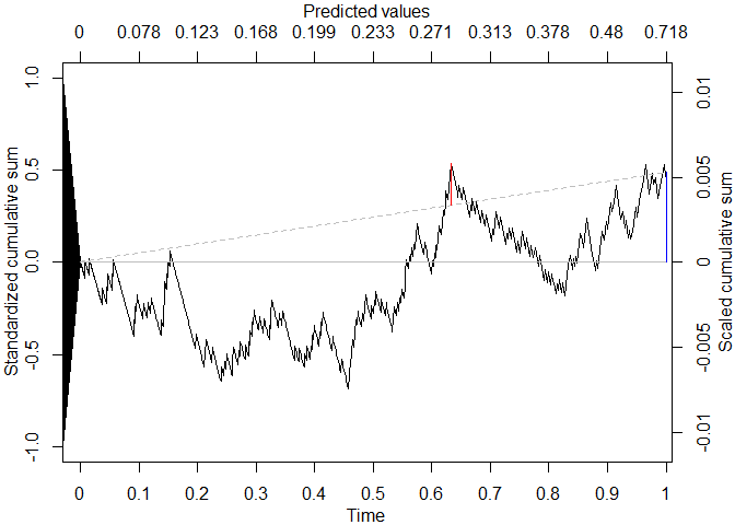
res <- cumulcalib(y, p)

summary(res)
#> C_n (mean calibration error): 0.00532270104567871
#> C* (maximum absolute cumulative calibration error): 0.00740996981029672
#> Method: Two-part Brownian Bridge (BB)
#> S_n (Z score for mean calibration error) 0.489295496431201
#> B* (test statistic for maximum absolute bridged calibration error): 0.904915434767163
#> Component-wise p-values: mean calibration=0.624632509005787 | Distance (bridged)=0.385979705481866
#> Combined p-value (Fisher's method): 0.584068794836004
#> Location of maximum drift: 812  | time value: 0.632911942275094  | predictor value: 0.28191196504736
plot(res, draw_sig=F)
