Description
Imputation Estimator from Borusyak, Jaravel, and Spiess (2021).
Description
Estimates Two-way Fixed Effects difference-in-differences/event-study models using the imputation-based approach proposed by Borusyak, Jaravel, and Spiess (2021).
README.md
didimputation
The goal of didimputation is to estimate TWFE models without running into the problem of staggered treatment adoption.
Installation
You can install didimputation from github with:
devtools::install_github("kylebutts/didimputation")
TWFE vs. DID Imputation Example
I will load example data from the package and plot the average outcome among the groups. Here is one unit’s data:
library(didimputation)
#> Loading required package: fixest
#> Loading required package: data.table
library(fixest)
library(ggplot2)

# Load Data from did2s package
data("df_het", package = "didimputation")
setDT(df_het)
Here is a plot of the average outcome variable for each of the groups:
# Plot Data
df_avg <- df_het[,
  .(dep_var = mean(dep_var)),
  by = .(group, year)
]

# Get treatment years for plotting
gs <- df_het[treat == TRUE, unique(g)]

ggplot() +
  geom_line(data = df_avg, mapping = aes(y = dep_var, x = year, color = group), size = 1.5) +
  geom_vline(xintercept = gs - 0.5, linetype = "dashed") +
  theme_minimal(base_size = 16) +
  theme(legend.position = "bottom") +
  labs(y = "Outcome", x = "Year", color = "Treatment Cohort") +
  scale_y_continuous(expand = expansion(add = .5)) +
  scale_color_manual(values = c("Group 1" = "#d2382c", "Group 2" = "#497eb3", "Group 3" = "#8e549f"))
#> Warning: Using `size` aesthetic for lines was deprecated in ggplot2 3.4.0.
#> ℹ Please use `linewidth` instead.
#> This warning is displayed once every 8 hours.
#> Call `lifecycle::last_lifecycle_warnings()` to see where this warning was
#> generated.
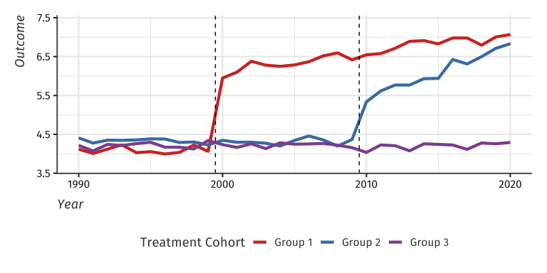
Example data with heterogeneous treatment effects
Estimate DID Imputation
First, lets estimate a static did:
# Static
static <- did_imputation(data = df_het, yname = "dep_var", gname = "g", tname = "year", idname = "unit")

static
#>      term estimate  std.error conf.low conf.high
#>    <char>    <num>      <num>    <num>     <num>
#> 1:  treat 2.262952 0.03139684 2.201414   2.32449
This is very close to the true treatment effect of 2.2384912.
Then, let’s estimate an event study did:
# Event Study
es <- did_imputation(
  data = df_het, yname = "dep_var", gname = "g",
  tname = "year", idname = "unit",
  # event-study
  horizon = TRUE, pretrends = -5:-1
)

es
#>       term    estimate  std.error    conf.low  conf.high
#>     <char>       <num>      <num>       <num>      <num>
#>  1:     -5 -0.06412085 0.07634962 -0.21376611 0.08552441
#>  2:     -4 -0.01201577 0.07634962 -0.16166103 0.13762949
#>  3:     -3 -0.01387197 0.07634962 -0.16351723 0.13577329
#>  4:     -2  0.05103140 0.07634962 -0.09861386 0.20067666
#>  5:     -1  0.02022464 0.07634962 -0.12942062 0.16986990
#>  6:      0  1.51314201 0.07547736  1.36520639 1.66107763
#>  7:      1  1.66384318 0.07675141  1.51341041 1.81427594
#>  8:      2  1.86436720 0.07450151  1.71834424 2.01039015
#>  9:      3  1.91872093 0.07471704  1.77227552 2.06516633
#> 10:      4  1.87322387 0.07418170  1.72782773 2.01862001
#> 11:      5  1.87844597 0.07567190  1.73012905 2.02676290
#> 12:      6  2.14373139 0.07632691  1.99413065 2.29333213
#> 13:      7  2.23777696 0.07610842  2.08860445 2.38694946
#> 14:      8  2.33650066 0.07446268  2.19055381 2.48244751
#> 15:      9  2.34352836 0.07471679  2.19708345 2.48997326
#> 16:     10  2.53443351 0.08109550  2.37548633 2.69338068
#> 17:     11  2.47944533 0.11953547  2.24515580 2.71373486
#> 18:     12  2.63493727 0.11531779  2.40891439 2.86096014
#> 19:     13  2.94449757 0.11047299  2.72797052 3.16102462
#> 20:     14  2.78171206 0.11466367  2.55697127 3.00645285
#> 21:     15  2.71470743 0.12030494  2.47890975 2.95050510
#> 22:     16  2.88065382 0.11563154  2.65401601 3.10729163
#> 23:     17  2.99383855 0.11438496  2.76964404 3.21803306
#> 24:     18  2.64616896 0.11545789  2.41987148 2.87246643
#> 25:     19  2.87530636 0.11405840  2.65175189 3.09886082
#> 26:     20  2.90465651 0.11320219  2.68278023 3.12653280
#>       term    estimate  std.error    conf.low  conf.high
And plot the results:
pts <- es |>
  as.data.table() |>
  DT(, .(rel_year = term, estimate, std.error)) |>
  DT(, let(
    ci_lower = estimate - 1.96 * std.error,
    ci_upper = estimate + 1.96 * std.error,
    group = "DID Imputation Estimate",
    rel_year = as.numeric(rel_year)
  ))

te_true <- df_het |>
  DT(
    g > 0,
    .(estimate = mean(te + te_dynamic)),
    by = "rel_year"
  ) |>
  DT(, group := "True Effect")

pts <- rbind(pts, te_true, fill = TRUE)

pts <- pts |>
  DT(rel_year >= -5 & rel_year <= 7, ) |>
  DT(, rel_year := ifelse(group == "DID Imputation Estimate", rel_year - 0.1, rel_year))

max_y <- max(pts$estimate)

ggplot() +
  # 0 effect
  geom_hline(yintercept = 0, linetype = "dashed") +
  geom_vline(xintercept = -0.5, linetype = "dashed") +
  # Confidence Intervals
  geom_linerange(data = pts, mapping = aes(x = rel_year, ymin = ci_lower, ymax = ci_upper), color = "grey30") +
  # Estimates
  geom_point(data = pts, mapping = aes(x = rel_year, y = estimate, color = group), size = 2) +
  # Label
  geom_label(
    data = data.frame(x = -0.5 - 0.1, y = max_y + 0.25, label = "Treatment Starts ▶"), label.size = NA,
    mapping = aes(x = x, y = y, label = label), size = 5.5, hjust = 1, fontface = 2, inherit.aes = FALSE
  ) +
  scale_x_continuous(breaks = -8:8, minor_breaks = NULL) +
  scale_y_continuous(minor_breaks = NULL) +
  scale_color_manual(values = c("DID Imputation Estimate" = "steelblue", "True Effect" = "#b44682")) +
  labs(x = "Relative Time", y = "Estimate", color = NULL, title = NULL) +
  theme_minimal(base_size = 16) +
  theme(legend.position = "bottom")
#> Warning: Removed 13 rows containing missing values (`geom_segment()`).
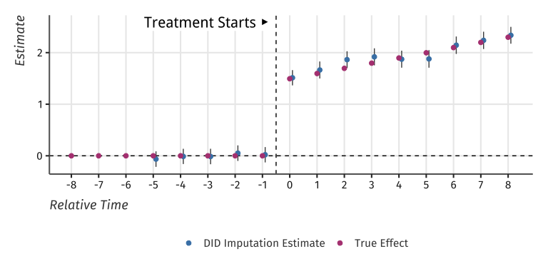
Event-study plot with example data
Comparison to TWFE
# TWFE
twfe <- fixest::feols(dep_var ~ i(rel_year, ref = c(-1, Inf)) | unit + year, data = df_het)

twfe_est <- broom::tidy(twfe)

twfe_est <- twfe_est |>
  DT(grepl("rel_year::", term)) |>
  DT(, .(rel_year = term, estimate, std.error)) |>
  DT(, let(
    rel_year = as.numeric(gsub("rel_year::", "", rel_year)),
    ci_lower = estimate - 1.96 * std.error,
    ci_upper = estimate + 1.96 * std.error,
    group = "TWFE Estimate"
  )) |>
  DT(rel_year >= -5 & rel_year <= 7, ) |>
  DT(, rel_year := rel_year + 0.1)

# Add TWFE Points
both_pts <- rbind(pts, twfe_est, fill = TRUE)

max_y <- max(pts$estimate)

ggplot() +
  # 0 effect
  geom_hline(yintercept = 0, linetype = "dashed") +
  geom_vline(xintercept = -0.5, linetype = "dashed") +
  # Confidence Intervals
  geom_linerange(data = both_pts, mapping = aes(x = rel_year, ymin = ci_lower, ymax = ci_upper), color = "grey30") +
  # Estimates
  geom_point(data = both_pts, mapping = aes(x = rel_year, y = estimate, color = group), size = 2) +
  # Label
  geom_label(
    data = data.frame(x = -0.5 - 0.1, y = max_y + 0.25, label = "Treatment Starts ▶"), label.size = NA,
    mapping = aes(x = x, y = y, label = label), size = 5.5, hjust = 1, fontface = 2, inherit.aes = FALSE
  ) +
  scale_x_continuous(breaks = -8:8, minor_breaks = NULL) +
  scale_y_continuous(minor_breaks = NULL) +
  scale_color_manual(values = c("DID Imputation Estimate" = "steelblue", "True Effect" = "#b44682", "TWFE Estimate" = "#82b446")) +
  labs(x = "Relative Time", y = "Estimate", color = NULL, title = NULL) +
  theme_minimal(base_size = 16) +
  theme(legend.position = "bottom")
#> Warning: Removed 13 rows containing missing values (`geom_segment()`).
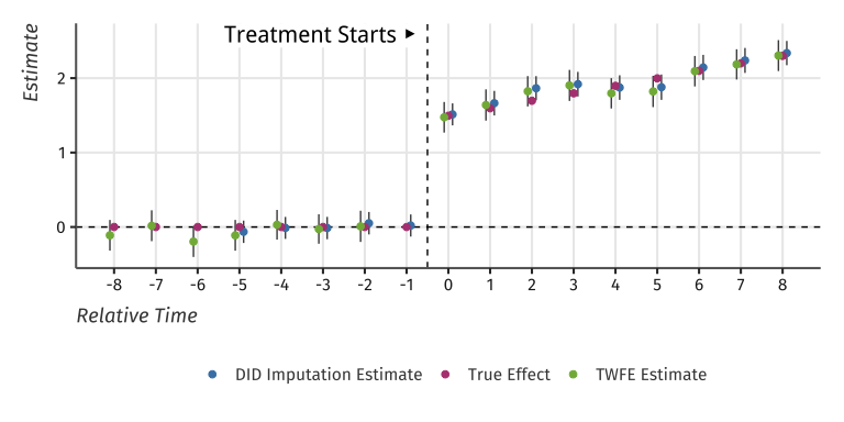
TWFE and Two-Stage estimates of Event-Study