Extended Changes-in-Changes.

Extended Changes-in-Changes (ECIC)

ecic estimates a changes-in-changes model with multiple periods and cohorts as suggested in Athey and Imbens (2006). Changes-in-changes is a generalization of the difference-in-differences approach, estimating a treatment effect for the entire distribution instead of averages.

Athey and Imbens (2006) show how to extend the model to multiple periods and cohorts, analogously to a two-way fixed-effects model for averages. This package implements this, calculating standard errors via bootstrap and plotting results, aggregated or in an event-study-style fashion.

Installation

ecic is available on CRAN using:

install.packages("ecic")

You can install the newest version from GitHub:

# install.packages("remotes")
remotes::install_github("frederickluser/ecic")

Basic Example

Estimation

Let's look at a short example how to use the package. First, load some simulated sample data.

library(ecic)
data(dat, package = "ecic")

head(dat)
#>  countyreal  first.treat   year time_to_treat   lemp
#>       <int>        <int>  <int>         <int>  <dbl>
#>           3        1980    1980             0   2.21
#>           3        1980    1981             1   3.33
#>           3        1980    1982             2   3.67
#>           5        1980    1980             0   2.77
#>           5        1980    1981             1   3.88
#>           5        1980    1982             2   3.80

Then, the function ecic estimates the changes-changes-model:

# Estimate the model
mod =
  ecic(
    yvar  = lemp,         # dependent variable
    gvar  = first.treat,  # group indicator
    tvar  = year,         # time indicator
    ivar  = countyreal,   # unit ID
    dat   = dat,          # dataset
    boot  = "weighted",   # bootstrap proceduce ("no", "normal", or "weighted")
    nReps = 10            # number of bootstrap runs
    )

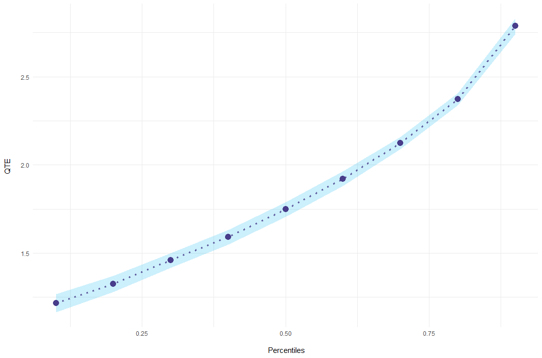
The input gvar denotes the period in which this individual receives the treatment. mod contains for every bootstrap run the point-estimates. The function summary then combines all bootstrap runs to a quantile treatment effect and adds standard errors:

mod_res = summary(mod) 

#> perc    coefs         se
#>  0.1 1.215531 0.02670761
#>  0.2 1.324130 0.02310521
#>  0.3 1.458270 0.02105119
#>  0.4 1.590848 0.02128534
#>  0.5 1.747296 0.02098057
#>  0.6 1.921818 0.02135982
#>  0.7 2.124138 0.01802972
#>  0.8 2.372483 0.01799869
#>  0.9 2.787395 0.02241811

Plotting

Finally, results can be plotted using ecic_plot.

ecic_plot(mod_res)

Event-Study Example

The package also allows to report event-study-style results of the effect. To do so, simply add the es = T argument to the estimation and summary will report effects for every event period.

# Estimate the model
mod =
  ecic(
    yvar  = lemp,         # dependent variable
    gvar  = first.treat,  # group indicator
    tvar  = year,         # time indicator
    ivar  = countyreal,   # unit ID
    dat   = dat,          # dataset
    es    = T,            # report an event study
    boot  = "weighted",   # bootstrap proceduce ("no", "normal", or "weighted")
    nReps = 10            # number of bootstrap runs
    )

# report results for every event period
mod_res = summary(mod) 

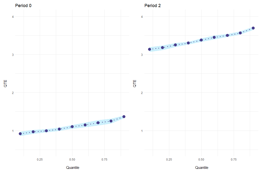
#> [[1]]
#> perc es     coefs         se
#>  0.1  0 0.9175263 0.02924326
#>  0.2  0 0.9675225 0.02508082
#>  0.3  0 0.9959150 0.02116782
#>  0.4  0 1.0388312 0.02373263
#>  0.5  0 1.0992322 0.02558309
#>  0.6  0 1.1496203 0.03078493
#>  0.7  0 1.2049797 0.03654320
#>  0.8  0 1.2519476 0.03291178
#>  0.9  0 1.3616626 0.01765538

#> [[2]]
#> perc es    coefs          se
#>  0.1  1 2.393816 0.022273736
#>  0.2  1 2.386941 0.020039276
#>  0.3  1 2.423415 0.017145110
#>  0.4  1 2.452259 0.017982620
#>  0.5  1 2.484616 0.009979006
#>  0.6  1 2.525388 0.012816760
#>  0.7  1 2.575615 0.015196499
#>  0.8  1 2.630959 0.019570320
#>  0.9  1 2.730742 0.024796025

#> [...]

Plotting

In addition to a standard plot showing everything at once, event-study results can be plotted for every period individually with the option es_type = "for_periods".

ecic_plot(
    mod_res, 
    periods_plot = c(0, 2),   # which periods you want to show
    es_type = "for_periods",  # plots by period
    ylim = c(.5, 4)           # same y-axis
    )

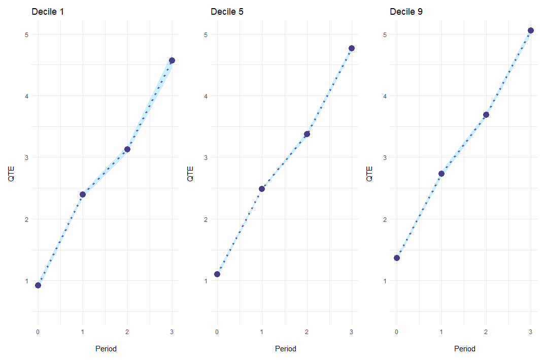
Alternatively, es_type = "for_quantiles" generates one plot for every quantile of interest.

ecic_plot(
    mod_res, 
    periods_plot = c(.1, .5, .9), # which quantiles you want to show
    es_type = "for_quantiles",    # plots by period
    ylim = c(.5, 5)               # same y-axis
    )

Under the hood

Estimation

For every treated cohort, we observe the distribution of the potential outcome $Y(1)$. In the case of two groups / cohorts and two periods, Athey and Imbens (2006) show how to construct the counterfactual $Y(0)$. This extends to the case with multiple cohorts and periods, where every not-yet-treated cohort is a valid comparison group. Hence, every combination of treated and not-yet-treated cohorts with a common pre-treatment period estimates in theory the quantile treatment effect. Then, I simply want to average them.

Yet, since it is not allowed to simply average quantile treatment effects, we must first store the empirical CDF of $Y(1)$ and $Y(0)$ for every two-by-two case. Next, I aggregate all estimated CDFs to get the plug-in estimates of $Y(1)$ and $Y(0)$, weighting for the cohort sizes. Finally, I invert them to get the quantile function and compute the quantile treatment effect as in the standard case.

Note that it is impossible to estimate a quantile treatment effect for units treated in the first (no pre-treatment period) and last period (no comparison cohort). In addition, the default value of nMin skips small cohorts (default nMin = 40) as we need more observations to estimate quantile treatment effects compared to an average effect.

Speed Improvements

Technically, ecic generates a grid over the dependent variable and imputes all empirical CDFs for every unique value of yvar. You can (cautiously) speed up the imputation by rounding the dependent variable to n_digits.

Bootstrap

I calculate standard errors by bootstrap. I resample with replacement the entire dataset and estimate $Y(1)$ and $Y(0)$ nRep times (default nReps = 1). Bootstrap can either be computed through replacement over the entire dataset (with boot = "normal") or you can weight by cohort sizes (with boot = "weighted") if you worry, for example, about small cohorts. This part can be parallelized by setting nCores > 1, speeding up the computation at the cost of additional overhead to load the cores.

progress_bar prints the progress of the bootstrapping by default. Alternatively, the option progress_bar = "cli" also shows estimated running time, but requires the cli package to be installed.

Next Steps for the package

• [ ] Add covariates.