Spatially Explicit Population Models of Disease Transmission in Wildlife.

epizootic

epizootic is an extension to poems, a spatially-explicit, process-explicit, pattern-oriented framework for modeling population dynamics. This extension adds functionality for modeling disease dynamics in wildlife. It also adds capability for seasonality and for unique dispersal dynamics for each life cycle stage.

Installation

You can install the latest release on CRAN with:

install.packages("epizootic")

You can install the latest version of epizootic from GitHub with:

# install.packages("devtools")
install.packages("poems")
devtools::install_github("viralemergence/epizootic")

Because epizootic is an extension to poems, it is necessary to install poems first.

About R6 classes

poems and epizootic run on R6 classes. R is primarily a functional programming language in which the primary units of programming are expressions and functions. Here we use R6 to create an object-oriented framework inside of R. R6 classes such as DiseaseModel and SimulationHandler are used to store model attributes, check them for consistency, pass them to parallel sessions for simulation, and gather results and errors.

Example

Here is the initial state of an idealized theoretical disease scenario, following a SIR disease model with three life cycle stages: juvenile, yearling, and adult.

library(poems)
library(purrr)
library(epizootic)
example_region <- Region$new(coordinates = data.frame(x = rep(seq(177.01, 177.05, 0.01), 5),
                             y = rep(seq(-18.01, -18.05, -0.01), each = 5)))
initial_abundance <- c(c(5000, 5000, 5000, 1, 0, 0, 0, 0, 0),
                          rep(c(5000, 5000, 5000, 0, 0, 0, 0, 0, 0), 24)) |>
      matrix(nrow = 9)
example_region$raster_from_values(initial_abundance[3,]) |>
  raster::plot(main = "Susceptible Adults")

example_region$raster_from_values(initial_abundance[4,]) |>
  raster::plot(main = "Infected Juveniles")

Here I create a DiseaseModel object, which stores inputs for disease simulations and checks them for consistency and completeness.

model_inputs <- DiseaseModel$new(
  time_steps = 10,
    seasons = 2,
    populations = 25,
    stages = 3,
    compartments = 3, # indicates disease compartments
    region = example_region,
    initial_abundance = initial_abundance,
    # Dimensions of carrying_capacity are populations by timesteps
    carrying_capacity = matrix(100000, nrow = 25, ncol = 10),
    # Indicates length of breeding season in days for each population
    breeding_season_length = rep(100, 25),
    # One mortality value for each stage and compartment
    mortality = c(0.4, 0.2, 0, 0.505, 0.25, 0.105, 0.4, 0.2, 0),
    # Indicates that these are seasonal mortality values
    mortality_unit = 1,
    # No reproduction in this simple example
    fecundity = 0,
    fecundity_unit = 1,
    fecundity_mask = rep(0, 9),
    # Transmission rates from infected individuals, one for each stage
    transmission = c(0.00002, 0.00001, 7.84e-06),
    # Indicates that these are daily transmission rates
    transmission_unit = 0,
    # Indicates that all stages in the first compartment, S, can be infected
    transmission_mask = c(1, 1, 1, 0, 0, 0, 0, 0, 0),
    recovery = c(0.05714286, 0.06, 0.1),
    recovery_unit = 0,
    # Indicates that all stages in the second compartment, I, can recover
    recovery_mask = c(0, 0, 0, 1, 1, 1, 0, 0, 0),
    season_functions = list(sir_model_summer, NULL), 
    dispersal = list(disperser),
    simulation_order = list(c("transition", "season_functions", "results"),
                            c("dispersal", "results")),
    verbose = F
)
model_inputs$is_complete()
#> [1] TRUE
model_inputs$is_consistent()
#> [1] TRUE

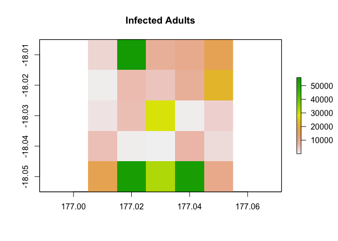
The core simulation engine of epizootic is the function disease_simulator, which simulates spatially explicit disease dynamics in populations. Here I show the results from the non-breeding season in the tenth year of the simulation.

results <- disease_simulator(model_inputs)
results$abundance_segments$stage_3_compartment_1[,10,2] |>
  example_region$raster_from_values() |>
  raster::plot(main = "Susceptible Adults")

results$abundance_segments$stage_3_compartment_2[,10,2] |>  
  example_region$raster_from_values() |>
  raster::plot(main = "Infected Adults")