Fast and Stable Fitting of Generalized Linear Models using 'RcppEigen'.

Overview of ‘fastglm’

The ‘fastglm’ package is a re-write of glm() using RcppEigen designed to be computationally efficient and algorithmically stable.

Installing the ‘fastglm’ package

Install the development version using the devtools package:

devtools::install_github("jaredhuling/fastglm")

or by cloning and building using R CMD INSTALL

Quick Usage Overview

Load the package:

library(fastglm)

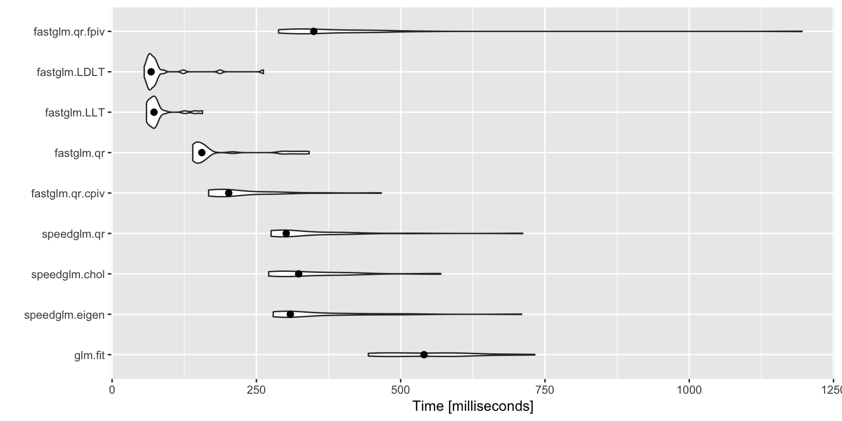
A (not comprehensive) comparison with glm.fit() and speedglm.wfit():

library(speedglm)
library(microbenchmark)
library(ggplot2)

set.seed(123)
n.obs  <- 10000
n.vars <- 100
x <- matrix(rnorm(n.obs * n.vars, sd = 3), n.obs, n.vars)
Sigma <- 0.99 ^ abs(outer(1:n.vars, 1:n.vars, FUN = "-"))
x <- MASS::mvrnorm(n.obs, mu = runif(n.vars, min = -1), Sigma = Sigma)

y <- 1 * ( drop(x[,1:25] %*% runif(25, min = -0.1, max = 0.10)) > rnorm(n.obs))

ct <- microbenchmark(
    glm.fit = {gl1 <- glm.fit(x, y, family = binomial())},
    speedglm.eigen  = {sg1 <- speedglm.wfit(y, x, intercept = FALSE,
                                            family = binomial())},
    speedglm.chol   = {sg2 <- speedglm.wfit(y, x, intercept = FALSE, 
                                            family = binomial(), method = "Chol")},
    speedglm.qr     = {sg3 <- speedglm.wfit(y, x, intercept = FALSE,
                                            family = binomial(), method = "qr")},
    fastglm.qr.cpiv = {gf1 <- fastglm(x, y, family = binomial())},
    fastglm.qr      = {gf2 <- fastglm(x, y, family = binomial(), method = 1)},
    fastglm.LLT     = {gf3 <- fastglm(x, y, family = binomial(), method = 2)},
    fastglm.LDLT    = {gf4 <- fastglm(x, y, family = binomial(), method = 3)},
    fastglm.qr.fpiv = {gf5 <- fastglm(x, y, family = binomial(), method = 4)},
    times = 25L
)

autoplot(ct, log = FALSE) + stat_summary(fun.y = median, geom = 'point', size = 2)

# comparison of estimates
c(glm_vs_fastglm_qrcpiv = max(abs(coef(gl1) - gf1$coef)),
  glm_vs_fastglm_qr     = max(abs(coef(gl1) - gf2$coef)),
  glm_vs_fastglm_qrfpiv = max(abs(coef(gl1) - gf5$coef)),
  glm_vs_fastglm_LLT    = max(abs(coef(gl1) - gf3$coef)),
  glm_vs_fastglm_LDLT   = max(abs(coef(gl1) - gf4$coef)))

## glm_vs_fastglm_qrcpiv     glm_vs_fastglm_qr glm_vs_fastglm_qrfpiv 
##          2.590289e-14          2.546921e-14          2.776945e-14 
##    glm_vs_fastglm_LLT   glm_vs_fastglm_LDLT 
##          1.140078e-13          1.094264e-13

# now between glm and speedglm
c(glm_vs_speedglm_eigen = max(abs(coef(gl1) - sg1$coef)),
  glm_vs_speedglm_Chol  = max(abs(coef(gl1) - sg2$coef)),
  glm_vs_speedglm_qr    = max(abs(coef(gl1) - sg3$coef)))

## glm_vs_speedglm_eigen  glm_vs_speedglm_Chol    glm_vs_speedglm_qr 
##          1.359413e-12          1.359413e-12          1.191977e-12

Stability

The fastglm package does not compromise computational stability for speed. In fact, for many situations where glm() and even glm2() do not converge, fastglm() does converge.

As an example, consider the following data scenario, where the response distribution is (mildly) misspecified, but the link function is quite badly misspecified. In such scenarios, the standard IRLS algorithm tends to have convergence issues. The glm2() package was designed to handle such cases, however, it still can have convergence issues. The fastglm() package uses a similar step-halving technique as glm2(), but it starts at better initialized values and thus tends to have better convergence properties in practice.

set.seed(1)
x <- matrix(rnorm(10000 * 100), ncol = 100)
y <- (exp(0.25 * x[,1] - 0.25 * x[,3] + 0.5 * x[,4] - 0.5 * x[,5] + rnorm(10000)) ) + 0.1


system.time(gfit1 <- fastglm(cbind(1, x), y, family = Gamma(link = "sqrt")))

##    user  system elapsed 
##   0.783   0.022   0.807

system.time(gfit2 <- glm(y~x, family = Gamma(link = "sqrt")) )

##    user  system elapsed 
##   3.035   0.121   3.166

system.time(gfit3 <- glm2::glm2(y~x, family = Gamma(link = "sqrt")) )

##    user  system elapsed 
##   2.117   0.084   2.205

system.time(gfit4 <- speedglm(y~x, family = Gamma(link = "sqrt")))

##    user  system elapsed 
##   1.757   0.048   1.807

## speedglm appears to diverge
system.time(gfit5 <- speedglm(y~x, family = Gamma(link = "sqrt"), maxit = 500))

##    user  system elapsed 
##  37.776   1.205  39.272

## Note that fastglm() returns estimates with the
## largest likelihood

c(fastglm = logLik(gfit1), glm = logLik(gfit2), glm2 = logLik(gfit3),
  speedglm = logLik(gfit4), speedglm500 = logLik(gfit5))

##     fastglm         glm        glm2    speedglm speedglm500 
##   -16030.81   -16704.05   -16046.66   -47722.66   -57785.72

rbind(fastglm     = coef(gfit1)[1:5],
      glm         = coef(gfit2)[1:5],
      glm2        = coef(gfit3)[1:5],
      speedglm    = coef(gfit4)[1:5],
      speedglm500 = coef(gfit5)[1:5])

##             (Intercept)          X1            X2         X3          X4
## fastglm        1.429256   0.1258736  5.321164e-03 -0.1293897   0.2389373
## glm            1.431168   0.1251936 -6.896739e-05 -0.1281857   0.2366473
## glm2           1.426864   0.1242616 -9.860241e-05 -0.1254873   0.2361301
## speedglm     -22.182477   3.1784570 -2.970111e+00 -4.9709797  14.0549438
## speedglm500  -27.891929 -13.9080256 -9.690833e+00  2.7279219 -11.1458325

## check convergence of fastglm and #iterations
# 1 means converged, 0 means not converged
c(gfit1$converged, gfit1$iter)

## [1]  1 17

## now check convergence for glm()
c(gfit2$converged, gfit2$iter)

## [1]  0 25

## check convergence for glm2()
c(gfit3$converged, gfit3$iter)

## [1]  1 19

## check convergence for speedglm()
c(gfit4$convergence, gfit4$iter, gfit5$convergence, gfit5$iter)

## [1]   0  25   0 500

## increasing number of IRLS iterations for glm() does not help that much
system.time(gfit2 <- glm(y~x, family = Gamma(link = "sqrt"), control = list(maxit = 1000)) )

##    user  system elapsed 
## 116.122   4.148 120.833

gfit2$converged

## [1] FALSE

gfit2$iter

## [1] 1000

logLik(gfit1)

## 'log Lik.' -16030.81 (df=102)

logLik(gfit2)

## 'log Lik.' -16333.99 (df=102)