Mean and Covariance Matrix Estimation under Heavy Tails.

fitHeavyTail

Robust estimation methods for the mean vector, scatter matrix, and covariance matrix (if it exists) from data (possibly containing NAs) under multivariate heavy-tailed distributions such as angular Gaussian (via Tyler's method), Cauchy, and Student's t distributions. Additionally, a factor model structure can be specified for the covariance matrix. The latest revision also includes the multivariate skewed t distribution.

Installation

The package can be installed from CRAN or GitHub:

# install stable version from CRAN
install.packages("fitHeavyTail")

# install development version from GitHub
devtools::install_github("convexfi/fitHeavyTail")

To get help:

library(fitHeavyTail)
help(package = "fitHeavyTail")
?fit_mvt

To cite fitHeavyTail in publications:

citation("fitHeavyTail")

Quick Start

To illustrate the simple usage of the package fitHeavyTail, let's start by generating some multivariate data under a Student's $t$ distribution with significant heavy tails (degrees of freedom $\nu=4$):

library(mvtnorm)  # package for multivariate t distribution
N <- 10   # number of variables
T <- 80   # number of observations
nu <- 4   # degrees of freedom for heavy tails

set.seed(42)
mu <- rep(0, N)
U <- t(rmvnorm(n = round(0.3*N), sigma = 0.1*diag(N)))
Sigma_cov <- U %*% t(U) + diag(N)  # covariance matrix with factor model structure
Sigma_scatter <- (nu-2)/nu * Sigma_cov
X <- rmvt(n = T, delta = mu, sigma = Sigma_scatter, df = nu)  # generate data

We can first estimate the mean vector and covariance matrix via the traditional sample estimates (i.e., sample mean and sample covariance matrix):

mu_sm     <- colMeans(X)
Sigma_scm <- cov(X)

Then we can compute the robust estimates via the package fitHeavyTail:

library(fitHeavyTail)
fitted <- fit_mvt(X)

We can now compute the estimation errors and see the significant improvement:

sum((mu_sm     - mu)^2)
#> [1] 0.2857323
sum((fitted$mu - mu)^2)
#> [1] 0.1487845

sum((Sigma_scm  - Sigma_cov)^2)
#> [1] 5.861138
sum((fitted$cov - Sigma_cov)^2)
#> [1] 4.663539

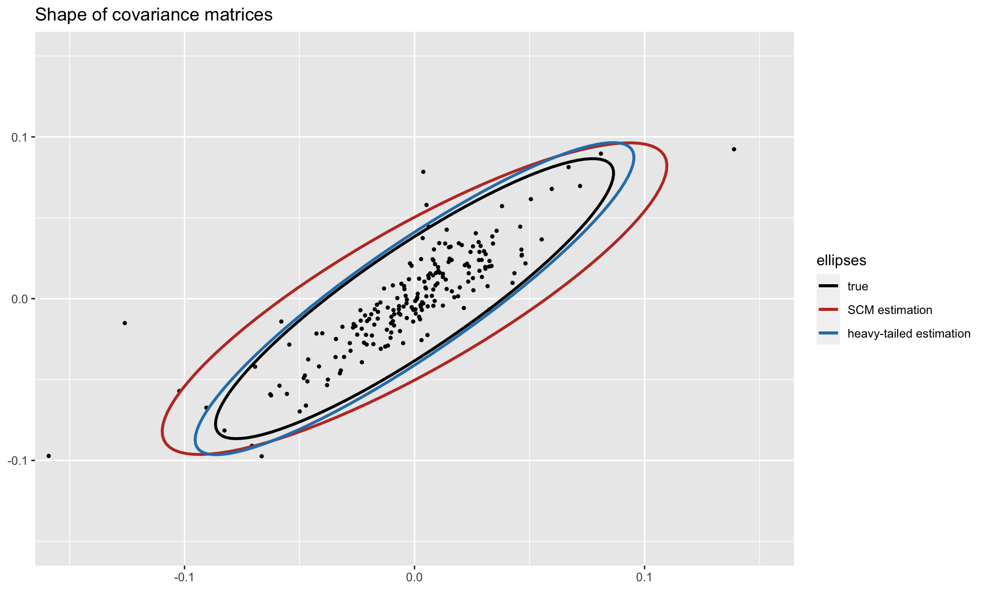
To get a visual idea of the robustness, we can plot the shapes of the covariance matrices (true and estimated ones) on two dimensions. Observe how the heavy-tailed estimation follows the true one more closely than the sample covariance matrix:

Documentation

For more detailed information, please check the vignette.

Links

Package: CRAN and GitHub.

README file: GitHub-readme.

Vignette: CRAN-vignette and GitHub-vignette.