Estimation of a Variety of Count Regression Models.
flexCountReg 
![]()
The goal of flexCountReg is to provide functions that allow the analyst to estimate count regression models that can handle multiple analysis issues including excess zeros, overdispersion as a function of variables (i.e., generalized count models), random parameters, etc.
Installation
You can install the development version of flexCountReg like using:
# install.packages("devtools")
devtools::install_github("jwood-iastate/flexCountReg")
Functions and Data
The following functions are included in the flexCountReg package, grouped by continuous and count distributions.
Distribution Functions
Continuous Distributions
Inverse Gamma Distribution
dinvgammafor the density functionpinvgammafor the cumulative density functionqinvgammafor the quantile functionrinvgammafor random number generation
Triangle Distribution
dtrifor the density functionptrifor the cumulative density functionqtrifor the quantile functionrtrifor random number generation
Lognormal Distribution
mgf_lognormalfor estimating the moment generating function
Count Distributions
Generalized Waring Distribution
dgwarfor the density functionpgwarfor the cumulative density functionqgwarfor the quantile functionrgwarfor random number generation
Poisson-Generalized-Exponential Distribution
dpgefor the density functionppgefor the cumulative density functionqpgefor the quantile functionrpgefor random number generation
Poisson-Inverse-Gaussian Distribution (Types 1 and 2)
dpinvgausfor the density functionppinvgausfor the cumulative density functionqpinvgausfor the quantile functionrpinvgausfor random number generation
Poisson-Inverse-Gamma Distribution
dpinvgammafor the density functionppinvgammafor the cumulative density functionqpinvgammafor the quantile functionrpinvgammafor random number generation
Poisson-Lindley Distribution
dplindfor the density functionpplindfor the cumulative density functionqplindfor the quantile functionrplindfor random number generation
Poisson-Lindley-Gamma (Negative Binomial-Lindley) Distribution
dplindGammafor the density functionpplindGammafor the cumulative density functionqplindGammafor the quantile functionrplindGammafor random number generation
Poisson-Lindley-Lognormal Distribution
dplindLnormfor the density functionpplindLnormfor the cumulative density functionqplindLnormfor the quantile functionrplindLnormfor random number generation
Poisson-Lognormal Distribution
dpLnormfor the density functionppLnormfor the cumulative density functionqtpLnormfor the quantile functionrpLnormfor random number generation
Poisson-Weibull Distribution
dpoisweibullfor the density functionppoisweibullfor the cumulative density functionqpoisweibullfor the quantile functionrpoisweibullfor random number generation
Sichel Distribution
dsichelfor the density functionpsichelfor the cumulative density functionqsichelfor the quantile functionrsichelfor random number generation
Conway-Maxwell-Poisson Distribution
dcomfor the density functionpcomfor the cumulative density functionqcomfor the quantile functionrcomfor random number generation
Model Estimation Functions
countregis a general function for estimating the non-panel, non-random parameters count regression modelscountreg.rpestimates the random parameters count models.poislind.reestimates the random effects Poisson-Lindley modelrenbestimates the random effects negative binomial regression model.
Model Evaluation, Comparison, and Convenience Functions
cureplotgenerates a CURE plot for the specified model, based on the cureplots package.maecomputes the Mean Absolute Error (MAE).myAICcomputes the Akaike Information Criterion (AIC) value.myBICcomputes the Bayesian Information Criterion (BIC) value.regCompTablecreates a publication-ready table comparing multiple models. This can include the regression estimate results, AIC, BIC, and Pseudo R-Square values.regCompTestcompares any given model with a base model. This can be used to perform a likelihood ratio test between models.rmsecomputes the Root Mean Squared Error (RMSE).predictallows the predict function to be used for out-of-sample predictions for any of the flexCountReg models.summaryallows the use of the summary function to get a model summary from a flexCountReg regression object.
Data A dataset, washington_roads, is included. It is based on a sample of Washington primary 2-lane roads from the years 2016-2018. Data for the roads, traffic volumes (AADT) and associated crashes were obtained from the Highway Safety Information System (HSIS).
Probability Distributions
As noted in the list of functions, the probability distributions below are included in the flexCountReg package. Details of the distributions are provided in the documentation (help files).
Continuous Distributions
- Inverse Gamma Distribution
- Triangle Distribution
Count DistributionsDistributions that Handle Equidispersion
- Poisson
Distributions that handle Underdispersion
- Conway-Maxwell-Poisson (COM) Distribution
Distributions that Handle Overdispersion
- Negative Binomial in various forms (NB-1, NB-2, and NB-P)
- Poisson-Inverse-Gaussian Distribution (Types 1 and 2)
- Poisson-Inverse-Gamma
- Poisson-Lognormal Distribution
- Poisson-Weibull Distribution
- Sichel Distribution
- Generalized Waring Distribution
Distributions that Handle Excess Zeros
- Poisson-Generalized-Exponential Distribution
- Poisson-Lindley Distribution
- Poisson-Lindley-Gamma (Negative Binomial-Lindley) Distribution
- Poisson-Lindley-Lognormal Distribution
Example
The following is an example of using flexCountReg to estimate a negative binomial (NB-2) regression model with the overdispersion parameter as a function of predictor variables:
library(gt) # used to format summary tables here
library(flexCountReg)
library(knitr)

data("washington_roads")
washington_roads$AADT10kplus <- ifelse(washington_roads$AADT > 10000, 1, 0)
gen.nb2 <- countreg(Total_crashes ~ lnaadt + lnlength + speed50 + AADT10kplus,
               data = washington_roads, family = "NB2",
               dis_param_formula_1 = ~ speed50,  method='BFGS')
kable(summary(gen.nb2), caption = "NB-2 Model Summary")
#> Call:
#>  Total_crashes ~ lnaadt + lnlength + speed50 + AADT10kplus
#>
#>  Method:  countreg
#> Iterations:  44
#> Convergence:  successful convergence
#> Log-likelihood:  -1064.876
#>
#> Parameter Estimates:
#> (Using bootstrapped standard errors)
#> # A tibble: 7 × 7
#>   parameter           coeff `Std. Err.` `t-stat` `p-value` `lower CI` `upper CI`
#>   <chr>               <dbl>       <dbl>    <dbl>     <dbl>      <dbl>      <dbl>
#> 1 (Intercept)        -7.40        0.043  -172.       0         -7.49      -7.32
#> 2 lnaadt              0.912       0.005   182.       0          0.902      0.921
#> 3 lnlength            0.843       0.037    22.9      0          0.771      0.915
#> 4 speed50            -0.47        0.102    -4.62     0         -0.669     -0.27
#> 5 AADT10kplus         0.77        0.089     8.61     0          0.594      0.945
#> 6 ln(alpha):(Interc… -1.62        0.291    -5.57     0         -2.19      -1.05
#> 7 ln(alpha):speed50   1.31        0.458     2.85     0.004      0.409      2.20
| parameter | coeff | Std. Err. | t-stat | p-value | lower CI | upper CI |
|---|---|---|---|---|---|---|
| (Intercept) | -7.401 | 0.043 | -171.562 | 0.000 | -7.486 | -7.317 |
| lnaadt | 0.912 | 0.005 | 182.453 | 0.000 | 0.902 | 0.921 |
| lnlength | 0.843 | 0.037 | 22.878 | 0.000 | 0.771 | 0.915 |
| speed50 | -0.470 | 0.102 | -4.619 | 0.000 | -0.669 | -0.270 |
| AADT10kplus | 0.770 | 0.089 | 8.607 | 0.000 | 0.594 | 0.945 |
| ln(alpha):(Intercept) | -1.619 | 0.291 | -5.568 | 0.000 | -2.189 | -1.049 |
| ln(alpha):speed50 | 1.306 | 0.458 | 2.854 | 0.004 | 0.409 | 2.203 |
NB-2 Model Summary
teststats <- regCompTest(gen.nb2)
kable(teststats$statistics)
| Statistic | Model | BaseModel |
|---|---|---|
| AIC | 2143.7522 | 3049.659 |
| BIC | 2180.9494 | 3054.973 |
| LR Test Statistic | 917.9070 | NA |
| LR degrees of freedom | 6.0000 | NA |
| LR p-value | 0.0000 | NA |
| McFadden’s Pseudo R^2 | 0.3012 | NA |
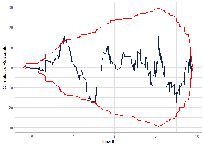
Checking the CURE plot:
cureplot(gen.nb2, indvar  ="lnaadt")
#> Covariate: indvar_values
#> CURE data frame was provided. Its first column, lnaadt, will be used.
Modifying the model to fit better:
gen.nb2 <- countreg(Total_crashes ~ lnaadt  + lnlength + speed50 +
                                ShouldWidth04 + AADT10kplus +
                                I(AADT10kplus/lnaadt),
                                data = washington_roads, family = "NB2",
                                dis_param_formula_1 = ~ lnlength,  method='BFGS')

kable(summary(gen.nb2), caption = "Modified NB-2 Model Summary")
#> Call:
#>  Total_crashes ~ lnaadt + lnlength + speed50 + ShouldWidth04 +      AADT10kplus + I(AADT10kplus/lnaadt)
#>
#>  Method:  countreg
#> Iterations:  56
#> Convergence:  successful convergence
#> Log-likelihood:  -1061.914
#>
#> Parameter Estimates:
#> (Using bootstrapped standard errors)
#> # A tibble: 9 × 7
#>   parameter           coeff `Std. Err.` `t-stat` `p-value` `lower CI` `upper CI`
#>   <chr>               <dbl>       <dbl>    <dbl>     <dbl>      <dbl>      <dbl>
#> 1 (Intercept)        -7.68        0.043  -180.       0         -7.76      -7.59
#> 2 lnaadt              0.93        0.005   188.       0          0.92       0.939
#> 3 lnlength            0.853       0.038    22.6      0          0.779      0.927
#> 4 speed50            -0.4         0.091    -4.38     0         -0.579     -0.221
#> 5 ShouldWidth04       0.261       0.06      4.36     0          0.143      0.378
#> 6 AADT10kplus         5.96        0.092    64.6      0          5.78       6.14
#> 7 I(AADT10kplus/ln… -50.1         0.938   -53.5      0        -52.0      -48.3
#> 8 ln(alpha):(Inter…  -1.91        0.324    -5.91     0         -2.55      -1.28
#> 9 ln(alpha):lnleng…  -0.43        0.244    -1.76     0.078     -0.908      0.048
| parameter | coeff | Std. Err. | t-stat | p-value | lower CI | upper CI |
|---|---|---|---|---|---|---|
| (Intercept) | -7.676 | 0.043 | -179.752 | 0.000 | -7.759 | -7.592 |
| lnaadt | 0.930 | 0.005 | 187.633 | 0.000 | 0.920 | 0.939 |
| lnlength | 0.853 | 0.038 | 22.585 | 0.000 | 0.779 | 0.927 |
| speed50 | -0.400 | 0.091 | -4.382 | 0.000 | -0.579 | -0.221 |
| ShouldWidth04 | 0.261 | 0.060 | 4.355 | 0.000 | 0.143 | 0.378 |
| AADT10kplus | 5.961 | 0.092 | 64.628 | 0.000 | 5.780 | 6.142 |
| I(AADT10kplus/lnaadt) | -50.133 | 0.938 | -53.454 | 0.000 | -51.971 | -48.295 |
| ln(alpha):(Intercept) | -1.913 | 0.324 | -5.910 | 0.000 | -2.547 | -1.278 |
| ln(alpha):lnlength | -0.430 | 0.244 | -1.764 | 0.078 | -0.908 | 0.048 |
Modified NB-2 Model Summary
teststats <- regCompTest(gen.nb2)
kable(teststats$statistics)
| Statistic | Model | BaseModel |
|---|---|---|
| AIC | 2141.8278 | 3049.659 |
| BIC | 2189.6528 | 3054.973 |
| LR Test Statistic | 923.8314 | NA |
| LR degrees of freedom | 8.0000 | NA |
| LR p-value | 0.0000 | NA |
| McFadden’s Pseudo R^2 | 0.3031 | NA |
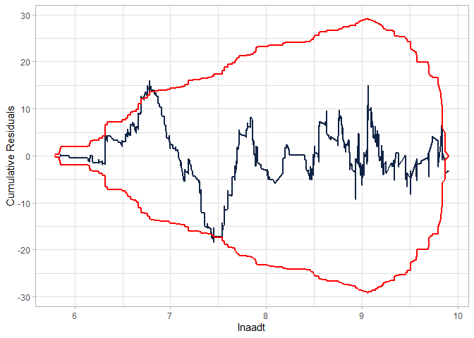
cureplot(gen.nb2, indvar  ="lnaadt")
#> Covariate: indvar_values
#> CURE data frame was provided. Its first column, lnaadt, will be used.
Estimating another model (NB-P) - without the interaction:
gen.nbp <- countreg(Total_crashes ~ lnaadt  + lnlength + speed50 +
                                ShouldWidth04 + AADT10kplus,
                                data = washington_roads, family = "NBp",
                                dis_param_formula_1 = ~ lnlength,  method='BFGS')
kable(summary(gen.nbp), caption = "NB-P Model Summary")
#> Call:
#>  Total_crashes ~ lnaadt + lnlength + speed50 + ShouldWidth04 +      AADT10kplus
#>
#>  Method:  countreg
#> Iterations:  53
#> Convergence:  successful convergence
#> Log-likelihood:  -1062.195
#>
#> Parameter Estimates:
#> (Using bootstrapped standard errors)
#> # A tibble: 9 × 7
#>   parameter           coeff `Std. Err.` `t-stat` `p-value` `lower CI` `upper CI`
#>   <chr>               <dbl>       <dbl>    <dbl>     <dbl>      <dbl>      <dbl>
#> 1 (Intercept)        -7.76        0.043 -181.        0         -7.85      -7.68
#> 2 lnaadt              0.938       0.005  189.        0          0.928      0.948
#> 3 lnlength            0.836       0.037   22.3       0          0.763      0.91
#> 4 speed50            -0.384       0.093   -4.13      0         -0.567     -0.202
#> 5 ShouldWidth04       0.258       0.059    4.34      0          0.141      0.374
#> 6 AADT10kplus         0.689       0.088    7.87      0          0.518      0.861
#> 7 ln(alpha):(Interc… -1.50        0.294   -5.09      0         -2.07      -0.92
#> 8 ln(alpha):lnlength -0.167       0.245   -0.682     0.495     -0.648      0.314
#> 9 ln(p)               0.525       0.173    3.03      0.002      0.186      0.864
| parameter | coeff | Std. Err. | t-stat | p-value | lower CI | upper CI |
|---|---|---|---|---|---|---|
| (Intercept) | -7.764 | 0.043 | -181.211 | 0.000 | -7.848 | -7.680 |
| lnaadt | 0.938 | 0.005 | 189.459 | 0.000 | 0.928 | 0.948 |
| lnlength | 0.836 | 0.037 | 22.314 | 0.000 | 0.763 | 0.910 |
| speed50 | -0.384 | 0.093 | -4.130 | 0.000 | -0.567 | -0.202 |
| ShouldWidth04 | 0.258 | 0.059 | 4.335 | 0.000 | 0.141 | 0.374 |
| AADT10kplus | 0.689 | 0.088 | 7.867 | 0.000 | 0.518 | 0.861 |
| ln(alpha):(Intercept) | -1.496 | 0.294 | -5.094 | 0.000 | -2.072 | -0.920 |
| ln(alpha):lnlength | -0.167 | 0.245 | -0.682 | 0.495 | -0.648 | 0.314 |
| ln(p) | 0.525 | 0.173 | 3.033 | 0.002 | 0.186 | 0.864 |
NB-P Model Summary
teststats <- regCompTest(gen.nbp)
kable(teststats$statistics)
| Statistic | Model | BaseModel |
|---|---|---|
| AIC | 2142.3895 | 3049.659 |
| BIC | 2190.2144 | 3054.973 |
| LR Test Statistic | 923.2697 | NA |
| LR degrees of freedom | 8.0000 | NA |
| LR p-value | 0.0000 | NA |
| McFadden’s Pseudo R^2 | 0.3029 | NA |
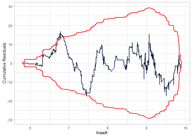
Checking the CURE plot (notice that the CURE plot is MUCH better in this case than the NB-2 without the interaction and still better than the modified NB-2):
cureplot(gen.nbp, indvar  ="lnaadt")
#> Covariate: indvar_values
#> CURE data frame was provided. Its first column, lnaadt, will be used.
Creating a table to compare the models:
regCompTable(list("Generalized NB-2"=gen.nb2, "Generalized NB-P"=gen.nbp), tableType="tibble") |>
  kable()
| Parameter | Generalized NB-2 | Generalized NB-P |
|---|---|---|
| (Intercept) | -7.676 (0.043)*** | -7.764 (0.043)*** |
| lnaadt | 0.93 (0.005)*** | 0.938 (0.005)*** |
| lnlength | 0.853 (0.038)*** | 0.836 (0.037)*** |
| speed50 | -0.4 (0.091)*** | -0.384 (0.093)*** |
| ShouldWidth04 | 0.261 (0.06)*** | 0.258 (0.059)*** |
| AADT10kplus | 5.961 (0.092)*** | 0.689 (0.088)*** |
| I(AADT10kplus/lnaadt) | -50.133 (0.938)*** | — |
| ln(alpha):(Intercept) | -1.913 (0.324)*** | -1.496 (0.294)*** |
| ln(alpha):lnlength | -0.43 (0.244) | -0.167 (0.245) |
| ln(p) | — | 0.525 (0.173)** |
| N Obs. | 1501 | 1501 |
| LL | -1061.914 | -1062.195 |
| AIC | 2141.828 | 2142.389 |
| BIC | 2189.653 | 2190.214 |
| Pseudo-R-Sq. | 0.303 | 0.303 |
Note that the metrics for comparison are similar. While the models both have the same number of parameters, the NB-P was able to get better performance without requiring the interaction terms (which leads to strange relationships between the exposure metric and the outcome).