Description

Functional Machine Learning Framework.

Description

A compact and explicit machine learning framework for supervised learning, resampling-based evaluation, hyperparameter tuning, learner comparison, interpretation, and plug-in g-computation. The package uses standard formulas for model specification and provides stable S3 interfaces for fitting, evaluation, tuning, interpretation, and causal estimation across a learner registry with multiple backend engines. Implemented interpretation methods build on established approaches such as permutation-based variable importance, partial dependence, individual conditional expectation, accumulated local effects, SHAP, and LIME; see Friedman (2001) <doi:10.1214/aos/1013203451>, Goldstein et al. (2015) <doi:10.1080/10618600.2014.907095>, Apley and Zhu (2020) <doi:10.1111/rssb.12377>, Lundberg and Lee (2017) <doi:10.48550/arXiv.1705.07874>, and Ribeiro et al. (2016) <doi:10.48550/arXiv.1602.04938>. The framework is intentionally opinionated: preprocessing is expected to occur outside the modeling step, and the API emphasizes explicit inputs, consistent object contracts, and compact interfaces rather than feature-by-feature competition with larger machine learning ecosystems.

README.md

cran.r-project.org

funcml

funcml is a functional machine learning framework for tabular data in R.

It provides one explicit interface for the core modeling workflow:

fit models with fit()
generate predictions with predict()
validate performance with evaluate()
tune hyperparameters with tune()
compare learners with compare_learners()
interpret fitted models with interpret()
estimate causal effects with estimate()

The package is intentionally compact and opinionated: preprocessing happens before modeling, inputs stay explicit, and the API stays small instead of expanding into a large orchestration layer.

Installation

install.packages("remotes")
remotes::install_github("ielbadisy/funcml")

Core API

The design of funcml centers on a small set of functions:

fit()
predict()
evaluate()
tune()
compare_learners()
interpret()
estimate()

Explore the registry

funcml exposes a session-aware registry of learners, metrics, and interpretation methods.

list_learners()
#>         learner   fit   predict   tune has_fit has_predict has_tune available
#> 15     adaboost fit() predict() tune()    TRUE        TRUE     TRUE      TRUE
#> 22         bart fit() predict() tune()    TRUE        TRUE     TRUE      TRUE
#> 9           C50 fit() predict() tune()    TRUE        TRUE     TRUE      TRUE
#> 18      cforest fit() predict() tune()    TRUE        TRUE     TRUE      TRUE
#> 17        ctree fit() predict() tune()    TRUE        TRUE     TRUE      TRUE
#> 6     e1071_svm fit() predict() tune()    TRUE        TRUE     TRUE      TRUE
#> 11        earth fit() predict() tune()    TRUE        TRUE     TRUE      TRUE
#> 14          fda fit() predict() tune()    TRUE        TRUE     TRUE      TRUE
#> 12          gam fit() predict() tune()    TRUE        TRUE     TRUE      TRUE
#> 8           gbm fit() predict() tune()    TRUE        TRUE     TRUE      TRUE
#> 1           glm fit() predict() tune()    TRUE        TRUE     TRUE      TRUE
#> 3        glmnet fit() predict() tune()    TRUE        TRUE     TRUE      TRUE
#> 10         kknn fit() predict() tune()    TRUE        TRUE     TRUE      TRUE
#> 19          lda fit() predict() tune()    TRUE        TRUE     TRUE      TRUE
#> 21     lightgbm fit() predict() tune()    TRUE        TRUE     TRUE      TRUE
#> 13   naivebayes fit() predict() tune()    TRUE        TRUE     TRUE      TRUE
#> 5          nnet fit() predict() tune()    TRUE        TRUE     TRUE      TRUE
#> 16          pls fit() predict() tune()    TRUE        TRUE     TRUE      TRUE
#> 20          qda fit() predict() tune()    TRUE        TRUE     TRUE      TRUE
#> 7  randomForest fit() predict() tune()    TRUE        TRUE     TRUE      TRUE
#> 4        ranger fit() predict() tune()    TRUE        TRUE     TRUE      TRUE
#> 2         rpart fit() predict() tune()    TRUE        TRUE     TRUE      TRUE
#> 24     stacking fit() predict() tune()    TRUE        TRUE     TRUE      TRUE
#> 25 superlearner fit() predict() tune()    TRUE        TRUE     TRUE      TRUE
#> 23      xgboost fit() predict() tune()    TRUE        TRUE     TRUE      TRUE

list_tunable_learners()
#>         learner   fit   predict   tune has_fit has_predict has_tune available
#> 15     adaboost fit() predict() tune()    TRUE        TRUE     TRUE      TRUE
#> 22         bart fit() predict() tune()    TRUE        TRUE     TRUE      TRUE
#> 9           C50 fit() predict() tune()    TRUE        TRUE     TRUE      TRUE
#> 18      cforest fit() predict() tune()    TRUE        TRUE     TRUE      TRUE
#> 17        ctree fit() predict() tune()    TRUE        TRUE     TRUE      TRUE
#> 6     e1071_svm fit() predict() tune()    TRUE        TRUE     TRUE      TRUE
#> 11        earth fit() predict() tune()    TRUE        TRUE     TRUE      TRUE
#> 14          fda fit() predict() tune()    TRUE        TRUE     TRUE      TRUE
#> 12          gam fit() predict() tune()    TRUE        TRUE     TRUE      TRUE
#> 8           gbm fit() predict() tune()    TRUE        TRUE     TRUE      TRUE
#> 1           glm fit() predict() tune()    TRUE        TRUE     TRUE      TRUE
#> 3        glmnet fit() predict() tune()    TRUE        TRUE     TRUE      TRUE
#> 10         kknn fit() predict() tune()    TRUE        TRUE     TRUE      TRUE
#> 19          lda fit() predict() tune()    TRUE        TRUE     TRUE      TRUE
#> 21     lightgbm fit() predict() tune()    TRUE        TRUE     TRUE      TRUE
#> 13   naivebayes fit() predict() tune()    TRUE        TRUE     TRUE      TRUE
#> 5          nnet fit() predict() tune()    TRUE        TRUE     TRUE      TRUE
#> 16          pls fit() predict() tune()    TRUE        TRUE     TRUE      TRUE
#> 20          qda fit() predict() tune()    TRUE        TRUE     TRUE      TRUE
#> 7  randomForest fit() predict() tune()    TRUE        TRUE     TRUE      TRUE
#> 4        ranger fit() predict() tune()    TRUE        TRUE     TRUE      TRUE
#> 2         rpart fit() predict() tune()    TRUE        TRUE     TRUE      TRUE
#> 24     stacking fit() predict() tune()    TRUE        TRUE     TRUE      TRUE
#> 25 superlearner fit() predict() tune()    TRUE        TRUE     TRUE      TRUE
#> 23      xgboost fit() predict() tune()    TRUE        TRUE     TRUE      TRUE

list_metrics()
#>               metric direction
#> 1               rmse  minimize
#> 2                mae  minimize
#> 3                mse  minimize
#> 4              medae  minimize
#> 5               mape  minimize
#> 6                rsq  maximize
#> 7           accuracy  maximize
#> 8          precision  maximize
#> 9             recall  maximize
#> 10       specificity  maximize
#> 11                f1  maximize
#> 12 balanced_accuracy  maximize
#> 13           logloss  minimize
#> 14             brier  minimize
#> 15               auc  maximize
#> 16      auc_weighted  maximize
#> 17               ece  minimize
#> 18               mce  minimize
#>                                                       summary     range
#> 1         Root mean squared error for regression predictions.  [0, Inf)
#> 2             Mean absolute error for regression predictions.  [0, Inf)
#> 3              Mean squared error for regression predictions.  [0, Inf)
#> 4           Median absolute error for regression predictions.  [0, Inf)
#> 5  Mean absolute percentage error for regression predictions.  [0, Inf)
#> 6    Coefficient of determination for regression predictions. (-Inf, 1]
#> 7                                    Classification accuracy.    [0, 1]
#> 8                    Macro-averaged classification precision.    [0, 1]
#> 9                       Macro-averaged classification recall.    [0, 1]
#> 10                 Macro-averaged classification specificity.    [0, 1]
#> 11                                   Macro-averaged F1 score.    [0, 1]
#> 12                          Macro-averaged balanced accuracy.    [0, 1]
#> 13  Negative log-likelihood for classification probabilities.  [0, Inf)
#> 14              Brier score for classification probabilities.    [0, 2]
#> 15                                  Area under the ROC curve.    [0, 1]
#> 16              Weighted multiclass area under the ROC curve.    [0, 1]
#> 17      Expected calibration error for binary classification.    [0, 1]
#> 18       Maximum calibration error for binary classification.    [0, 1]

list_interpretability_methods()
#>                                  compute   plot has_compute has_plot
#> 1              interpret(method = "vip") plot()        TRUE     TRUE
#> 2          interpret(method = "permute") plot()        TRUE     TRUE
#> 3              interpret(method = "pdp") plot()        TRUE     TRUE
#> 4              interpret(method = "ice") plot()        TRUE     TRUE
#> 5              interpret(method = "ale") plot()        TRUE     TRUE
#> 6            interpret(method = "local") plot()        TRUE     TRUE
#> 7             interpret(method = "lime") plot()        TRUE     TRUE
#> 8             interpret(method = "shap") plot()        TRUE     TRUE
#> 9      interpret(method = "local_model") plot()        TRUE     TRUE
#> 10     interpret(method = "interaction") plot()        TRUE     TRUE
#> 11       interpret(method = "surrogate") plot()        TRUE     TRUE
#> 12         interpret(method = "profile") plot()        TRUE     TRUE
#> 13 interpret(method = "ceteris_paribus") plot()        TRUE     TRUE
#> 14     interpret(method = "calibration") plot()        TRUE     TRUE

Example data

This README uses funcml::arthritis as the main running example.

Here, status is the outcome for a binary classification task.

demo_dat <- funcml::arthritis
demo_dat$status <- as.factor(demo_dat$status)
levels(demo_dat$status)
#> [1] "No"  "Yes"

Fit a classification model

fit() trains a model and returns a funcml_fit object.

xgb_spec <- list(
  nrounds = 30,
  max_depth = 3,
  eta = 0.1,
  subsample = 1,
  colsample_bytree = 1
)

fit_obj <- fit(
  status ~ age + gender + bmi + diabetes + smoke + covered_health,
  data = demo_dat,
  model = "xgboost",
  spec = xgb_spec,
  seed = 42
)

fit_obj
#> <funcml_fit> classification model: xgboost
#> Formula: status ~ age + gender + bmi + diabetes + smoke + covered_health
#> Features: 6 | Obs: 4856

Generate predictions

The same fitted object can produce class predictions or class probabilities.

predict(fit_obj, demo_dat[1:6, ])
#> [1] Yes No  No  No  No  No 
#> Levels: No Yes

pred_prob <- predict(
  fit_obj,
  demo_dat[1:6, ],
  type = "prob"
)

pred_prob
#>             No        Yes
#> [1,] 0.4382392 0.56176078
#> [2,] 0.5414010 0.45859897
#> [3,] 0.8288925 0.17110750
#> [4,] 0.9638367 0.03616334
#> [5,] 0.5076765 0.49232352
#> [6,] 0.5064105 0.49358952

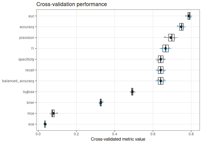
Evaluate predictive performance

evaluate() applies the same learner under a resampling plan and returns fold-level results with summary statistics.

eval_obj <- evaluate(
  data = demo_dat,
  formula = status ~ age + gender + bmi + diabetes + smoke + covered_health,
  model = "xgboost",
  spec = xgb_spec,
  resampling = cv(v = 4, seed = 42)
)

eval_obj
#> <funcml_eval> model: xgboost | task: classification
#>               metric       mean          sd n   std_error conf_level   conf_low
#> 1           accuracy 0.74732290 0.014617703 4 0.007308852       0.95 0.72406287
#> 2          precision 0.69316319 0.023420234 4 0.011710117       0.95 0.65589637
#> 3             recall 0.64049156 0.017832484 4 0.008916242       0.95 0.61211610
#> 4        specificity 0.64049156 0.017832484 4 0.008916242       0.95 0.61211610
#> 5                 f1 0.66573813 0.019521730 4 0.009760865       0.95 0.63467470
#> 6  balanced_accuracy 0.64049156 0.017832484 4 0.008916242       0.95 0.61211610
#> 7            logloss 0.49248120 0.008783385 4 0.004391692       0.95 0.47850488
#> 8              brier 0.32776953 0.007550594 4 0.003775297       0.95 0.31575485
#> 9                auc 0.78694529 0.011843752 4 0.005921876       0.95 0.76809924
#> 10               ece 0.03590688 0.004195513 4 0.002097757       0.95 0.02923089
#> 11               mce 0.08002388 0.013678803 4 0.006839402       0.95 0.05825786
#>     conf_high
#> 1  0.77058293
#> 2  0.73043001
#> 3  0.66886702
#> 4  0.66886702
#> 5  0.69680156
#> 6  0.66886702
#> 7  0.50645753
#> 8  0.33978421
#> 9  0.80579135
#> 10 0.04258288
#> 11 0.10178991

plot(eval_obj)

funcml also supports grouped cross-validation, time-based resampling, and holdout validation through group_cv(), time_cv(), and holdout().

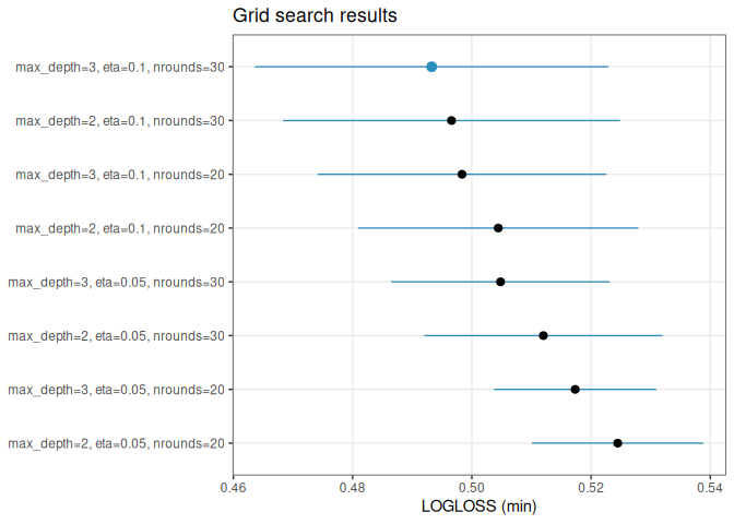
Tune hyperparameters

tune() searches candidate hyperparameter settings using the same evaluation framework.

tune_grid <- expand.grid(
  max_depth = c(2, 3),
  eta = c(0.05, 0.1),
  nrounds = c(20, 30)
)

tune_obj <- tune(
  data = demo_dat,
  formula = status ~ age + gender + bmi + diabetes + smoke + covered_health,
  model = "xgboost",
  grid = tune_grid,
  resampling = cv(v = 3, seed = 42),
  metric = "logloss",
  subsample = 1,
  colsample_bytree = 1,
  seed = 42
)

tune_obj
#> <funcml_tune> metric=logloss direction=min search=grid
#> Best:
#>   max_depth eta nrounds      mean       sd n   std_error conf_level conf_low
#> 8         3 0.1      30 0.4932667 0.011934 3 0.006890096       0.95 0.463621
#>   conf_high
#> 8 0.5229124

plot(tune_obj)

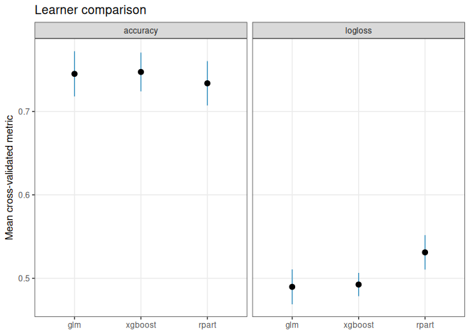
Compare learners

compare_learners() benchmarks multiple learners under a common resampling design.

compare_obj <- compare_learners(
  data = demo_dat,
  formula = status ~ age + gender + bmi + diabetes + smoke + covered_health,
  models = c("glm", "rpart", "xgboost"),
  metrics = c("accuracy", "logloss"),
  resampling = cv(v = 4, seed = 42),
  specs = list(xgboost = xgb_spec)
)

compare_obj
#> <funcml_compare> task: classification | tuned: FALSE
#>     model   metric      mean          sd n   std_error conf_level  conf_low
#> 1     glm accuracy 0.7450577 0.017034681 4 0.008517341       0.95 0.7179517
#> 2     glm  logloss 0.4897129 0.013140445 4 0.006570223       0.95 0.4688036
#> 3   rpart accuracy 0.7337315 0.016711299 4 0.008355649       0.95 0.7071401
#> 4   rpart  logloss 0.5310715 0.012975648 4 0.006487824       0.95 0.5104243
#> 5 xgboost accuracy 0.7473229 0.014617703 4 0.007308852       0.95 0.7240629
#> 6 xgboost  logloss 0.4924812 0.008783385 4 0.004391692       0.95 0.4785049
#>   conf_high tuned rank
#> 1 0.7721636 FALSE    2
#> 2 0.5106223 FALSE    1
#> 3 0.7603229 FALSE    3
#> 4 0.5517186 FALSE    3
#> 5 0.7705829 FALSE    1
#> 6 0.5064575 FALSE    2

plot(compare_obj)

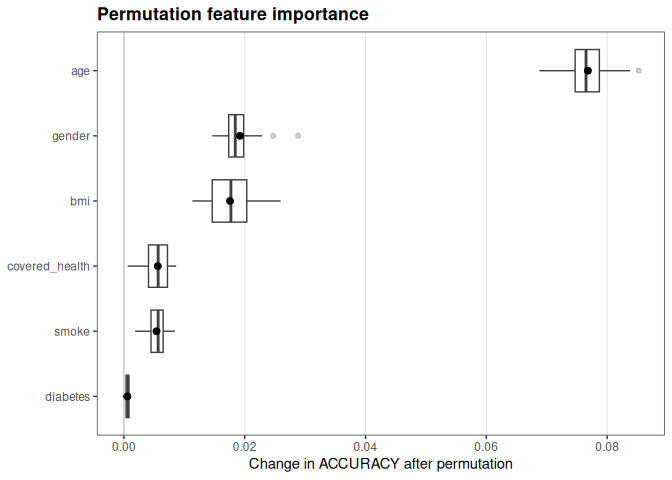
Interpret fitted models

interpret() operates directly on fitted funcml_fit objects.

permute_obj <- interpret(
  fit = fit_obj,
  data = demo_dat,
  method = "permute",
  nsim = 20,
  seed = 42
)

summary(permute_obj)
#>          feature   importance      std_dev
#> 1            age 0.0768121911 0.0039101175
#> 2         gender 0.0192030478 0.0032380942
#> 3            bmi 0.0175658979 0.0038212586
#> 4 covered_health 0.0056013180 0.0021176594
#> 5          smoke 0.0053953871 0.0017159311
#> 6       diabetes 0.0005663097 0.0003398597

plot(permute_obj)

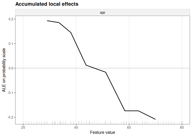
A second example shows accumulated local effects for one feature from the same fitted model.

ale_obj <- interpret(
  fit = fit_obj,
  data = demo_dat,
  method = "ale",
  features = c("age"),
  type = "prob"
)

plot(ale_obj)

Other supported methods include PDP, ICE, SHAP, local explanations, surrogate models, interaction diagnostics, and calibration plots.

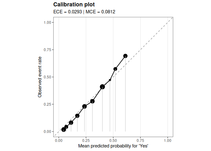
Inspect calibration

For classification, the same interface also supports calibration diagnostics.

calibration_obj <- interpret(
  fit = fit_obj,
  data = demo_dat,
  method = "calibration",
  type = "prob",
  bins = 10,
  strategy = "quantile"
)

plot(calibration_obj)

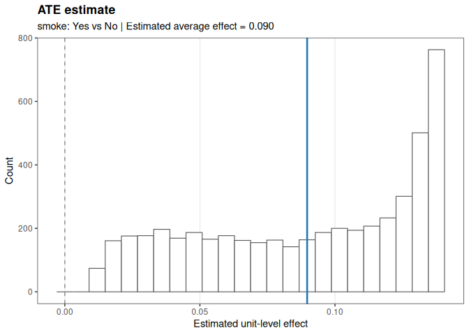
Estimate causal effects

estimate() extends the same framework to plug-in g-computation estimands such as the ATE.

The example below treats smoke as the treatment variable and status as the outcome, adjusting for the remaining covariates.

est_obj <- estimate(
  data = demo_dat,
  formula = status ~ smoke + diabetes + age + gender + bmi + covered_health,
  model = "glm",
  estimand = "ATE",
  treatment = "smoke",
  interval = "normal",
  seed = 42
)

est_obj
#> <funcml_estimand> ATE via g-computation
#> Treatment: smoke (Yes vs No)
#> Estimate: 0.0897 | SE: 0.0006 | 95% normal CI [0.0886, 0.0908]

plot(est_obj)

The same interface also supports ATT, CATE, and IATE.

Ensembles as first-class learners

Ensembles live in the same learner registry as base models.

stack_fit <- fit(
  status ~ age + gender + bmi + diabetes + smoke + covered_health,
  data = demo_dat,
  model = "superlearner", # or "stacking"
  spec = list(
    learners = c("glm", "rpart", "xgboost", "nnet"),
    learner_specs = list(xgboost = xgb_spec),
    meta_model = "glmnet"
  ),
  seed = 42
)

predict(stack_fit, demo_dat[1:5, ], type = "prob")
#>             No        Yes
#> [1,] 0.3184784 0.68152164
#> [2,] 0.5011472 0.49885283
#> [3,] 0.8758539 0.12414610
#> [4,] 0.9258312 0.07416884
#> [5,] 0.4985016 0.50149842

Summary

funcml provides a compact interface for tabular machine learning in R.

Use it to:

train models
generate predictions
validate performance
tune hyperparameters
compare learners
interpret fitted models
estimate causal effects

The package is designed to keep the main analysis workflow explicit.

Contributing

Contributions are welcome.

For development setup, coding standards, and pull request guidelines, see CONTRIBUTING.md.

Citation

If you use funcml in your work, cite the repository using GitHub’s Cite this repository panel or the metadata in CITATION.cff.

APA:

El Badisy, I. (2026). funcml (Version 0.7.1) [Computer software]. https://github.com/ielbadisy/funcml

BibTeX:

@software{El_Badisy_funcml_2026, author = {El Badisy, Imad}, 
license = {GPL-3.0-only},
month = apr,
title = {{funcml}},
url = {https://github.com/ielbadisy/funcml},
version = {0.7.1},
year = {2026}
}

r-funcml

funcml

Installation

Core API

Explore the registry

Example data

Fit a classification model

Generate predictions

Evaluate predictive performance

Tune hyperparameters

Compare learners

Interpret fitted models

Inspect calibration

Estimate causal effects

Ensembles as first-class learners

Summary

Contributing

Citation

Version

License

Status

Source

Homepage

Platforms (80)

funcml

Installation

Core API

Explore the registry

Example data

Fit a classification model

Generate predictions

Evaluate predictive performance

Tune hyperparameters

Compare learners

Interpret fitted models

Inspect calibration

Estimate causal effects

Ensembles as first-class learners

Summary

Contributing

Citation

Version

License

Status

Source

Homepage

Platforms80 (80)

Platforms (80)