Modern Graphs for Design of Experiments with 'ggplot2'.

ggDoE

Installation

You can install:

• the latest release from CRAN with

install.packages('ggDoE')

• the development version from GitHub with

if (!require("pak")) install.packages("pak")
pak::pak("toledo60/ggDoE")

Overview

With ggDoE you’ll be able to generate common plots used in Design of Experiments with ggplot2.

library(ggDoE)

The following plots are currently available:

1. Alias Matrix
2. Box-Cox Transformation
3. Lambda Plot
4. Boxplots
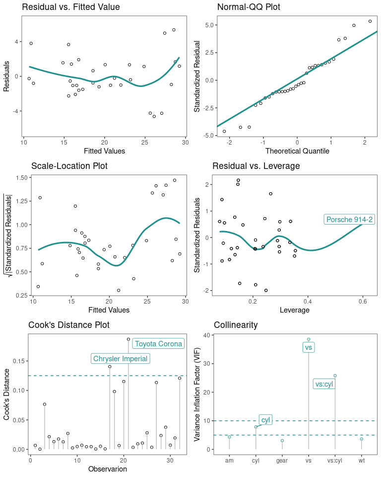
5. Regression Diagnostic Plots
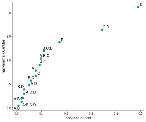
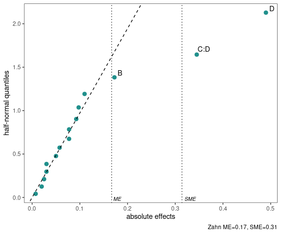
6. Half-Normal Plot
7. Interaction Effects Plot for a Factorial Design
8. Main Effects Plot for a Factorial Design
9. Contour Plots for Response Surface Methodology
10. Pareto Plot
11. Two Dimensional Projections of a Latin Hypercube Design

The following datasets/designs are included in ggDoE as tibbles:

• adapted_epitaxial: Adapted epitaxial layer experiment obtain from the book
  “Experiments: Planning, Analysis, and Optimization, 2nd Edition”

• original_epitaxial: Original epitaxial layer experiment obtain from the book
  “Experiments: Planning, Analysis, and Optimization, 2nd Edition”

• pulp_experiment: Reflectance Data, Pulp Experiment obtain from the book
  “Experiments: Planning, Analysis, and Optimization, 2nd Edition”

• girder_experiment: Girder experiment obtain from the book
  “Experiments: Planning, Analysis, and Optimization, 2nd Edition”

• aliased_design: D-efficient minimal aliasing design obtained from the article
  “Efficient Designs With Minimal Aliasing by Bradley Jones and Christopher J. Nachtsheim”

Citation

If you want to cite this package in a scientific journal or in any other context, run the following code in your R console

citation('ggDoE')

Warning in citation("ggDoE"): could not determine year for 'ggDoE' from package
DESCRIPTION file

To cite package 'ggDoE' in publications use:

  Toledo Luna J (????). _ggDoE: Modern Graphs for Design of Experiments
  with 'ggplot2'_. R package version 0.8, <https://ggdoe.netlify.app>.

A BibTeX entry for LaTeX users is

  @Manual{,
    title = {ggDoE: Modern Graphs for Design of Experiments with 'ggplot2'},
    author = {Jose {Toledo Luna}},
    note = {R package version 0.8},
    url = {https://ggdoe.netlify.app},
  }

Contributing to the package

I welcome feedback, suggestions, issues, and contributions! Check out the CONTRIBUTING file for more details.

Examples of Plots

Alias Matrix

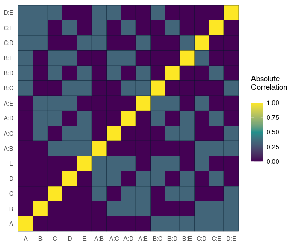
Correlation matrix plot to visualize the Alias matrix

alias_matrix(design=aliased_design)

Box-Cox Transformation

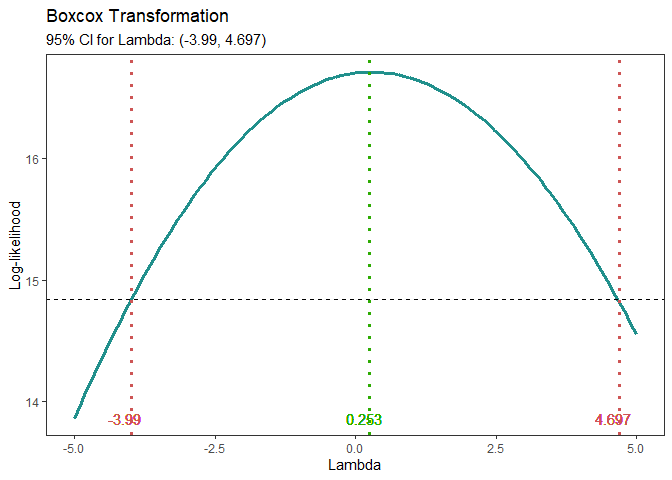
model <- lm(s2 ~ (A+B+C+D),data = adapted_epitaxial)
boxcox_transform(model,lambda = seq(-5,5,0.2))

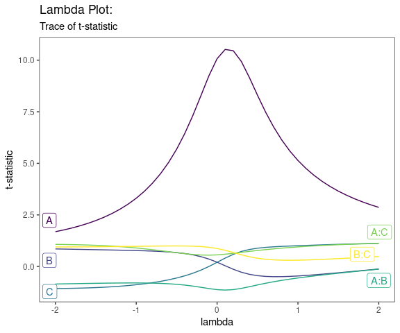
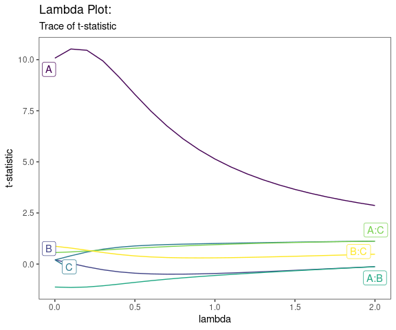
Lambda Plot

Obtain the trace plot of the t-statistics after applying Boxcox transformation across a specified sequence of lambda values

model <-  lm(s2 ~ (A+B+C)^2,data=original_epitaxial)
lambda_plot(model)

lambda_plot(model, lambda = seq(0,2,by=0.1))

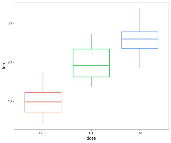
Boxplots

data <- ToothGrowth
data$dose <- factor(data$dose,levels = c(0.5, 1, 2),
                    labels = c("D0.5", "D1", "D2"))

gg_boxplots(data,y = 'len',x = 'dose')

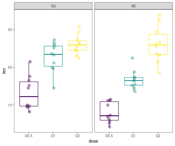
gg_boxplots(data,y = 'len',x = 'dose',
            group_var = 'supp',
            color_palette = 'viridis',
            jitter_points = TRUE)

Regression Diagnostic Plots

1. Residual vs. Fitted Values
2. Normal-QQ plot
3. Scale-Location plot
4. Residual vs. Leverage
5. Cook’s Distance
6. Collinearity

The default plots are 1-4

model <- lm(mpg ~ wt + am + gear + vs * cyl, data = mtcars)
gg_lm(model,which_plots=1:6)

Half-Normal Plot

model <- lm(ybar ~ (A+B+C+D)^4,data=adapted_epitaxial)
half_normal(model)

half_normal(model,method='Zahn',alpha=0.1,
            ref_line=TRUE,label_active=TRUE,
            margin_errors=TRUE)

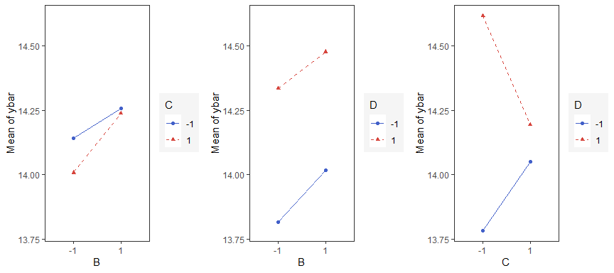
Interaction Effects Plot

Interaction effects plot between two factors in a factorial design

interaction_effects(adapted_epitaxial,response = 'ybar',
                    exclude_vars = c('s2','lns2'))

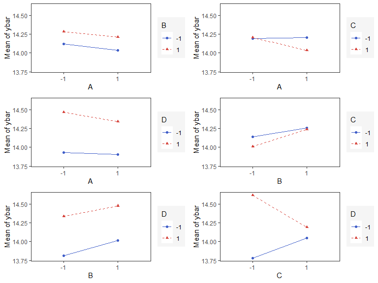
interaction_effects(adapted_epitaxial,response = 'ybar',
                    exclude_vars = c('A','s2','lns2'),
                    n_columns=3)

Main Effects Plots

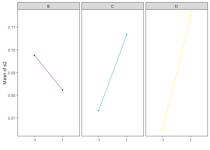
Main effect plots for each factor in a factorial design

main_effects(original_epitaxial,
             response='s2',
             exclude_vars = c('A','ybar','lns2'),
             color_palette = 'viridis',
             n_columns=3)

Contour Plots

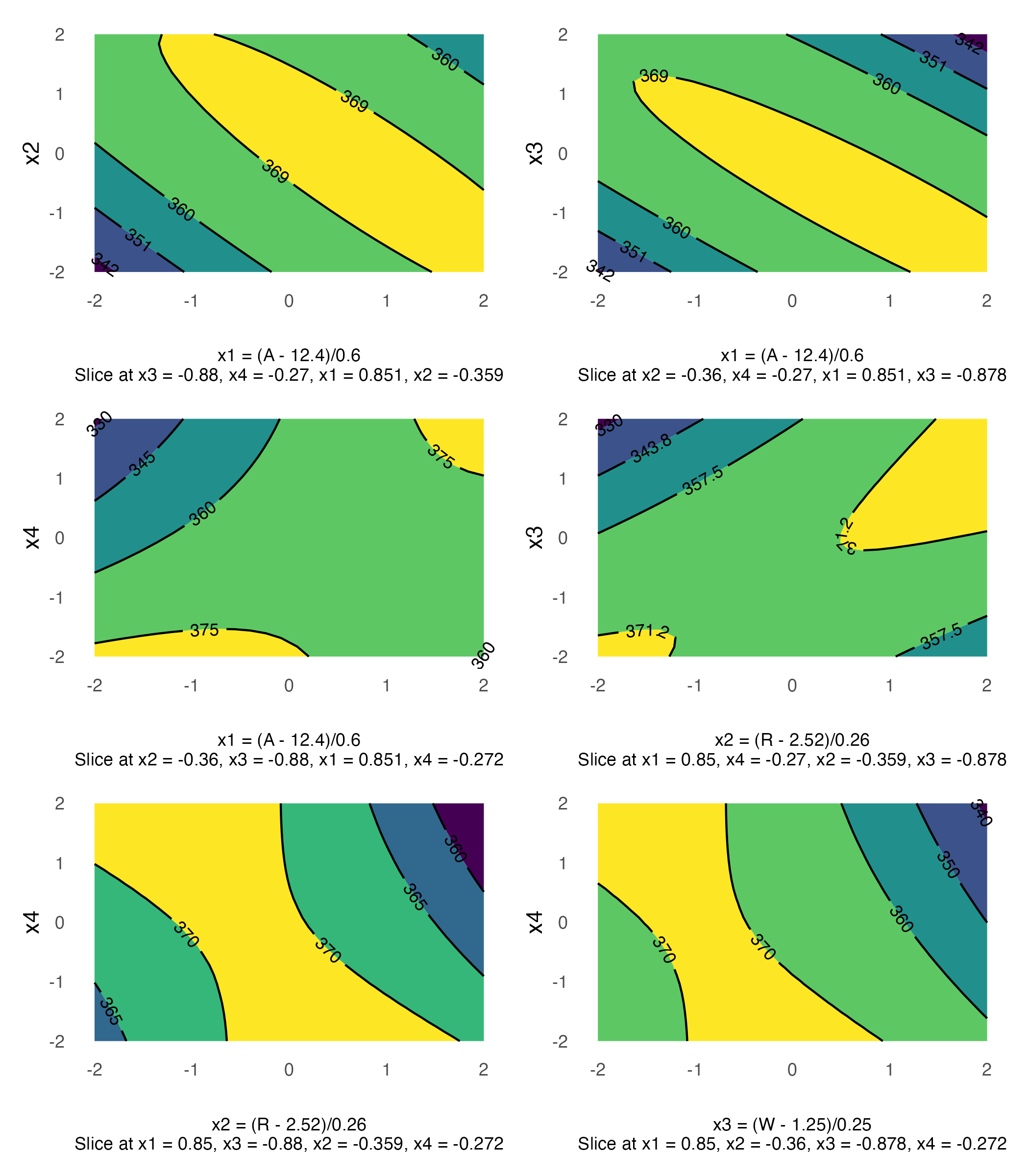
contour plot(s) that display the fitted surface for an rsm object involving two or more numerical predictors

heli.rsm <- rsm::rsm(ave ~ SO(x1, x2, x3, x4), 
                     data = rsm::heli)

gg_rsm(heli.rsm,formula = ~x1+x2+x3+x4,
       at = rsm::xs(heli.rsm))

Pareto Plot

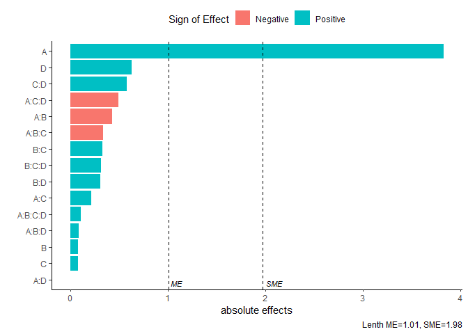
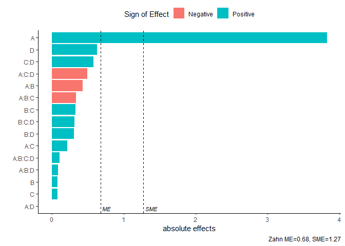
Pareto plot of effects with cutoff values for the margin of error (ME) and simultaneous margin of error (SME)

model <- lm(lns2 ~ (A+B+C+D)^4,data=original_epitaxial)
pareto_plot(model)

pareto_plot(model,method='Zahn',alpha=0.1)

Two Dimensional Projections

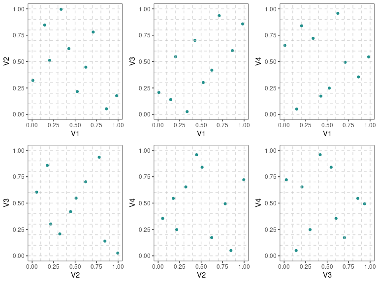
This function will output all two dimensional projections from a Latin hypercube design

set.seed(10)
X <- lhs::randomLHS(n=10, k=4)
pair_plots(X,n_columns=3,grid = TRUE)