Grab Bag of 'ggplot2' Functions.

ggallin

If you think I'm into this for the money you're dead wrong because I'm not doing this for the money. I'm doing it because it lives inside of me. -- GG Allin

A grab bag of ggplot2 extensions and hacks.

-- Steven E. Pav, [email protected]

Installation

This package can be installed from CRAN (not yet), via drat, or from github:

# via CRAN: (not yet)
# install.packages("ggallin")
# via drat:
if (require(drat)) {
    drat:::add("shabbychef")
    install.packages("ggallin")
}
# get snapshot from github (may be buggy)
if (require(devtools)) {
  install_github('shabbychef/ggallin')
}

geom_cloud

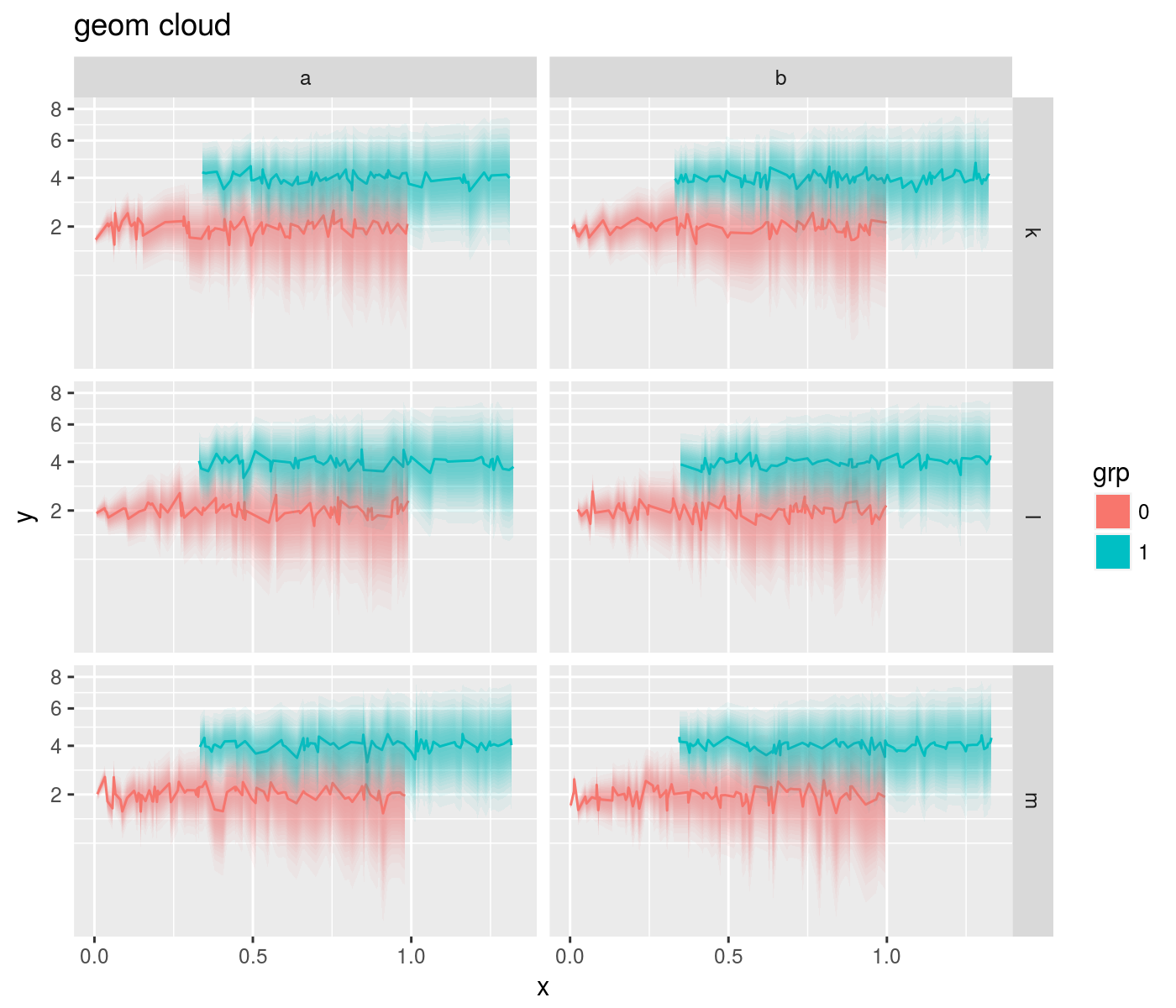
This geom acts nearly as a drop-in replacement for geom_errorbar, converting ymin and ymax into 'clouds' of uncertainty with alpha proportional to normal density.

library(ggplot2)
library(ggallin)
library(dplyr)

nobs <- 1000

set.seed(2134)
mydat <- data.frame(grp=sample(c(0,1),nobs,replace=TRUE),
                    colfac=sample(letters[1:2],nobs,replace=TRUE),
                    rowfac=sample(letters[10 + (1:3)],nobs,replace=TRUE)) %>%
  mutate(x=seq(0,1,length.out=nobs) + 0.33 * grp) %>%
  mutate(y=0.25*rnorm(nobs) + 2*grp) %>%
  mutate(grp=factor(grp)) %>%
  mutate(se=sqrt(x)) %>%
  mutate(ymin=y-se,ymax=y+se)

offs <- 2
ph <- mydat %>%
  mutate(y=y+offs,ymin=ymin+offs,ymax=ymax+offs) %>%
  ggplot(aes(x=x,y=y,ymin=ymin,ymax=ymax,color=grp,fill=grp)) + 
  facet_grid(rowfac ~ colfac) +
  scale_y_sqrt() + geom_line() + 
  geom_cloud(aes(fill=grp),steps=15,max_alpha=0.85,color=NA) +   
  labs(title='geom cloud')
print(ph)

log-like transforms

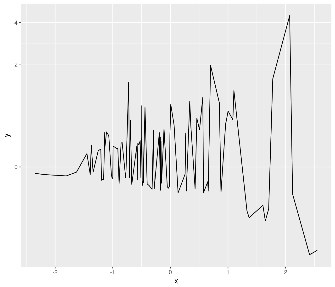
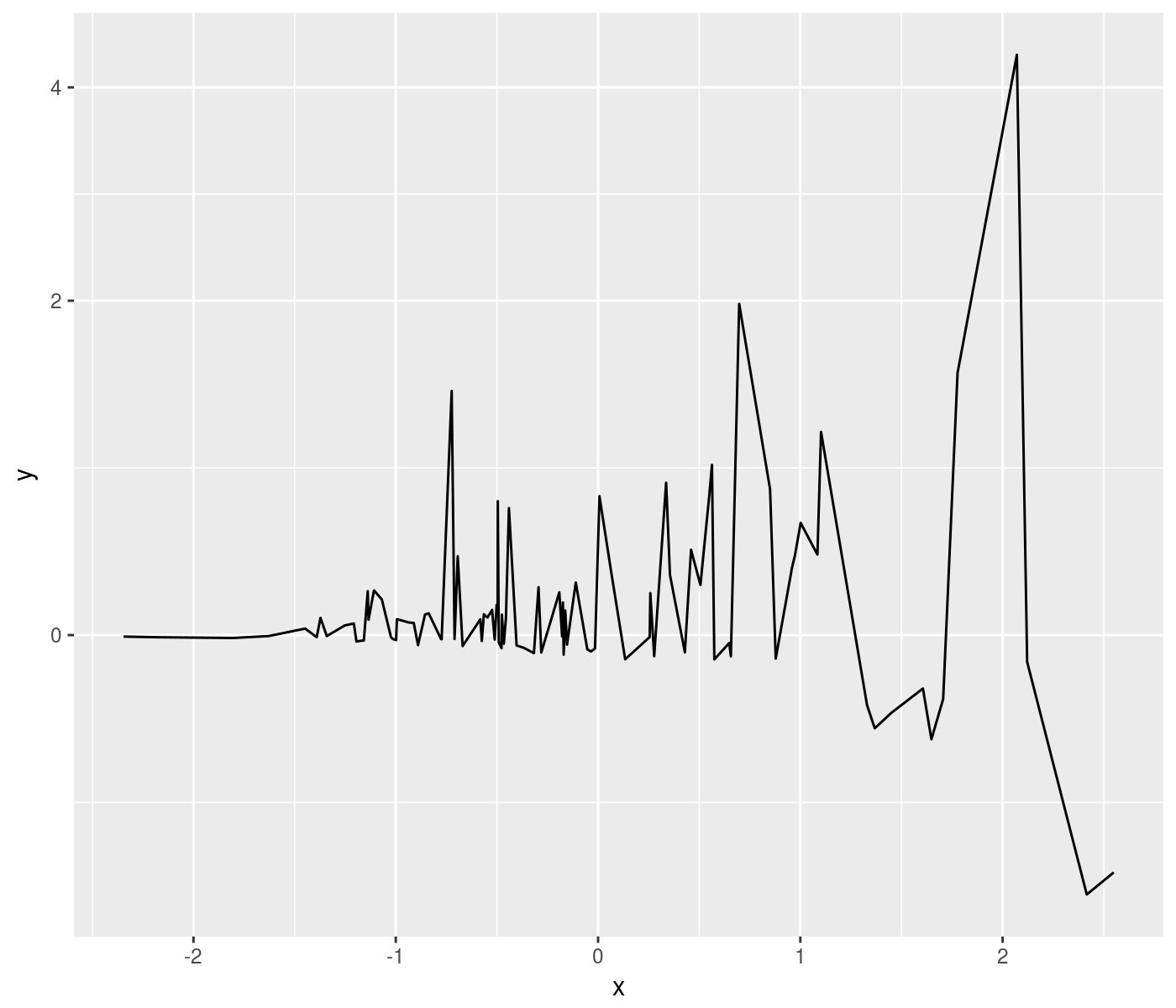
The square root transform is a good compromise between raw and logarithmic scales, showing detail across different scales without over-emphasizing very small variation. However, it does not work for negative numbers. Thus a signed square root transform is useful. Along similar lines, the pseudo-log transform accepts negative numbers while providing a good view across magnitudes. Some illustrations:

library(ggplot2)
library(ggallin)
library(dplyr)

nobs <- 100

# this is a silly example, don't blame me
set.seed(1234)
mydat <- data.frame(x=rnorm(nobs),z=rnorm(nobs)) %>%
  mutate(y=sign(z) * exp(x+z-2)) 
ph <- mydat %>%
  ggplot(aes(x=x,y=y)) + 
  geom_line() + 
  scale_y_continuous(trans=ssqrt_trans)
print(ph)

ph <- mydat %>%
  ggplot(aes(x=x,y=y)) + 
  geom_line() + 
  scale_y_continuous(trans=pseudolog10_trans)
print(ph)

interpolated transforms

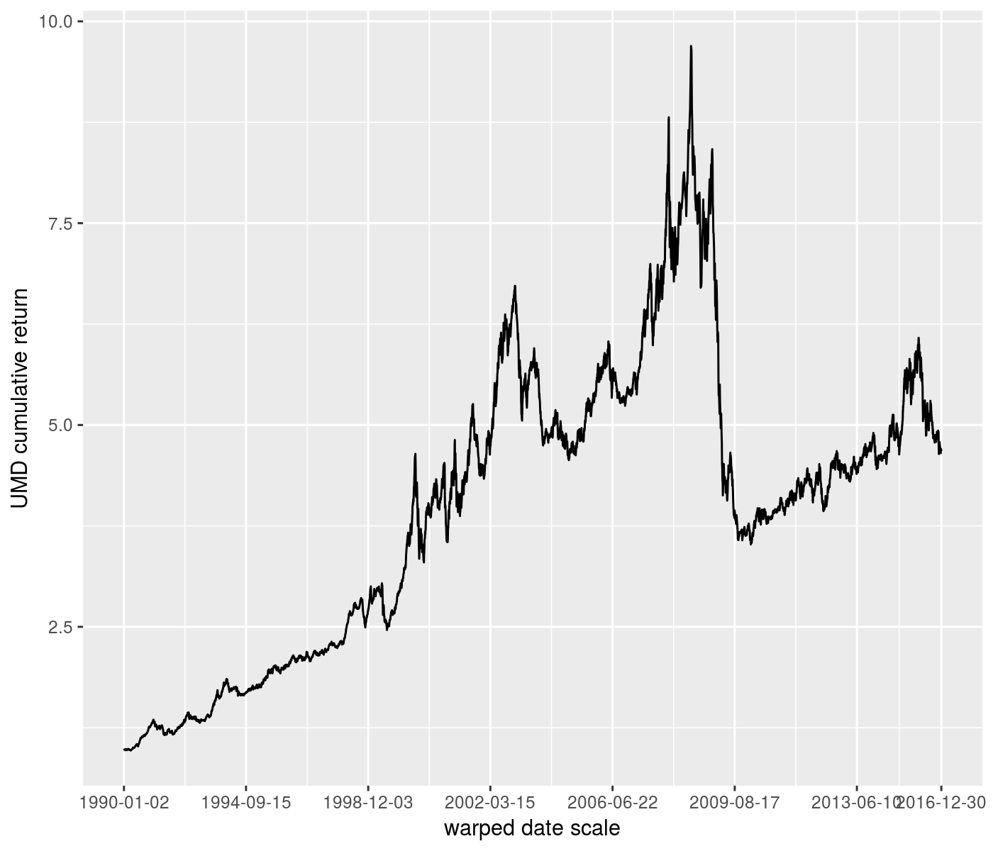
Scale transforms are useful for 'straightening out' crooked data graphically. Sometimes these transforms can not be expressed functionally but instead rely on data. In this case we can imagine that we have some paired data that provide the transformation x -> y. We provide a scale transformation that supports linear interpolation. We also provide another scale transformation that accepts x and positive 'weights' w, and computes y by taking the cumulative sum of weights, called a 'warp' transformation.

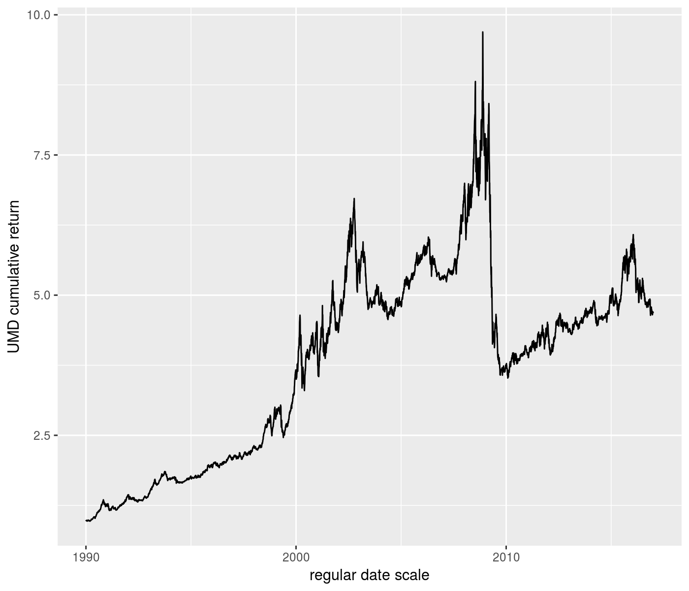
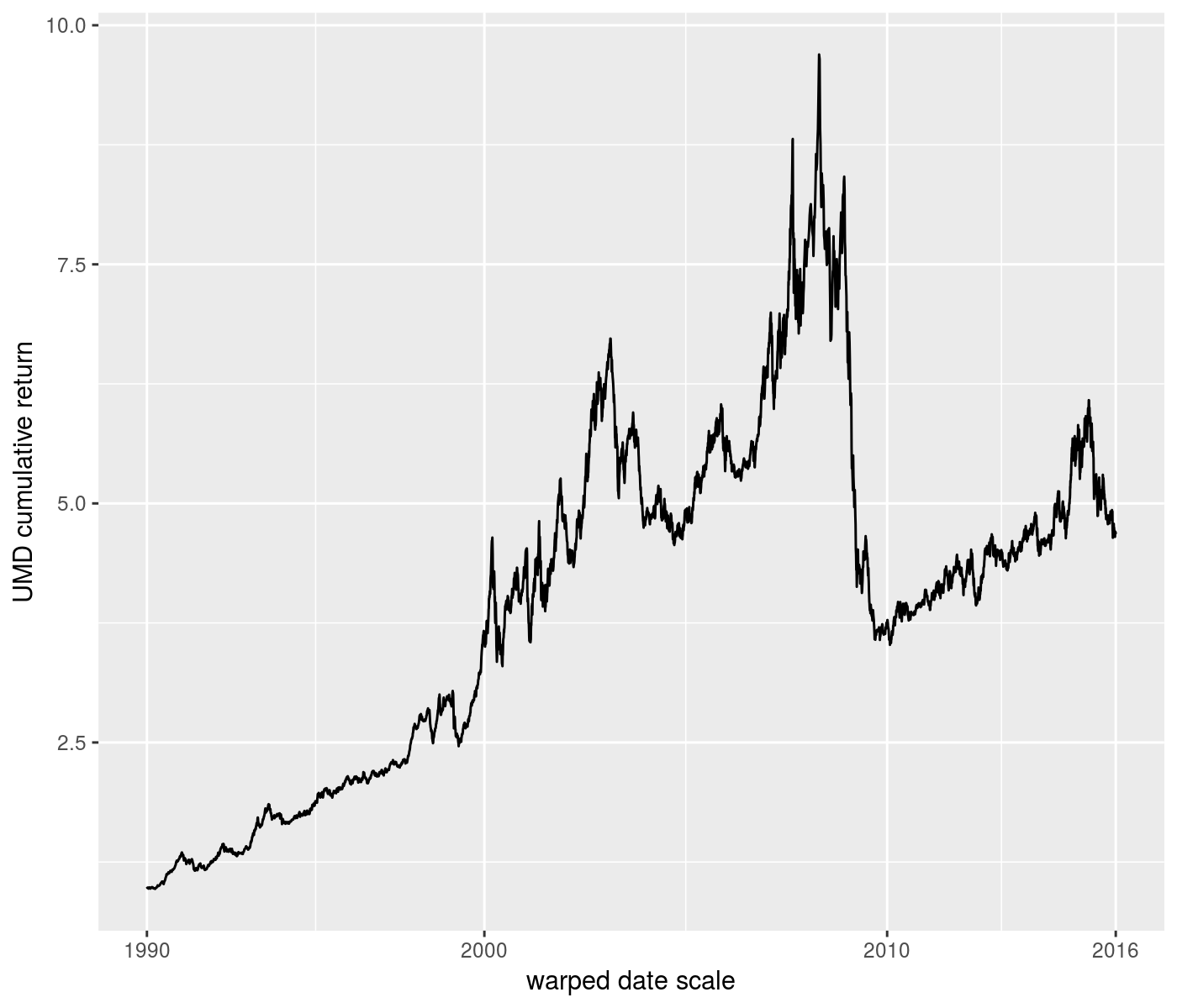
Here we illustrate the warp transformation by plotting the cumulative return of the 'UMD' factor against a time scale that is uniform in cumulative daily VIX (whatever that means):

library(ggplot2)
library(ggallin)
library(dplyr)
library(aqfb.data)
library(scales)

data(dvix)
data(dff4)

rr_to_nav <- function(x) {
  exp(cumsum(log(1 + x)))
}

rets <- dff4 %>%
  as.data.frame() %>%
  tibble::rownames_to_column(var='date') %>%
  inner_join(dvix %>%
             as.data.frame() %>%
             setNames(c('VIX')) %>%
             tibble::rownames_to_column(var='date'),by='date') %>%
  mutate(date=as.Date(date,format='%Y-%m-%d')) %>%
  mutate(UMD_nav=rr_to_nav(0.01*UMD),
         SMB_nav=rr_to_nav(0.01*SMB),
         HML_nav=rr_to_nav(0.01*HML))

  ph <- rets %>%
    ggplot(aes(x=date,y=UMD_nav)) +
    geom_line() +
    labs(y='UMD cumulative return') + 
    labs(x='regular date scale')
  print(ph)

  # select breaks automagically
  ph <- rets %>%
    ggplot(aes(x=date,y=UMD_nav)) +
    geom_line() + 
    scale_x_continuous(trans=warp_trans(x=rets$date,w=rets$VIX)) +
    labs(y='UMD cumulative return') + 
    labs(x='warped date scale')
  print(ph)

  # force decade breaks:
  ph <- rets %>%
    ggplot(aes(x=date,y=UMD_nav)) +
    geom_line() + 
    scale_x_continuous(trans=warp_trans(x=rets$date,w=rets$VIX,
                                        breaks=scales::date_breaks('10 years'),
                                        format=scales::date_format('%Y'))) +
labs(y='UMD cumulative return') + 
labs(x='warped date scale')
print(ph)

# reverse scale as well (see composition of transforms)
ph <- rets %>%
  ggplot(aes(x=date,y=UMD_nav)) +
  geom_line() + 
  scale_x_continuous(trans=scales::reverse_trans() %of% warp_trans(x=rets$date,w=rets$VIX)) +
  labs(y='UMD cumulative return') + 
  labs(x='reversed, warped date scale')
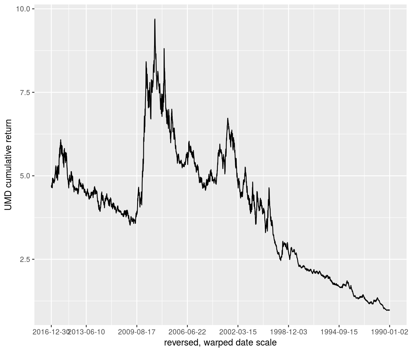
print(ph)

composition of transforms

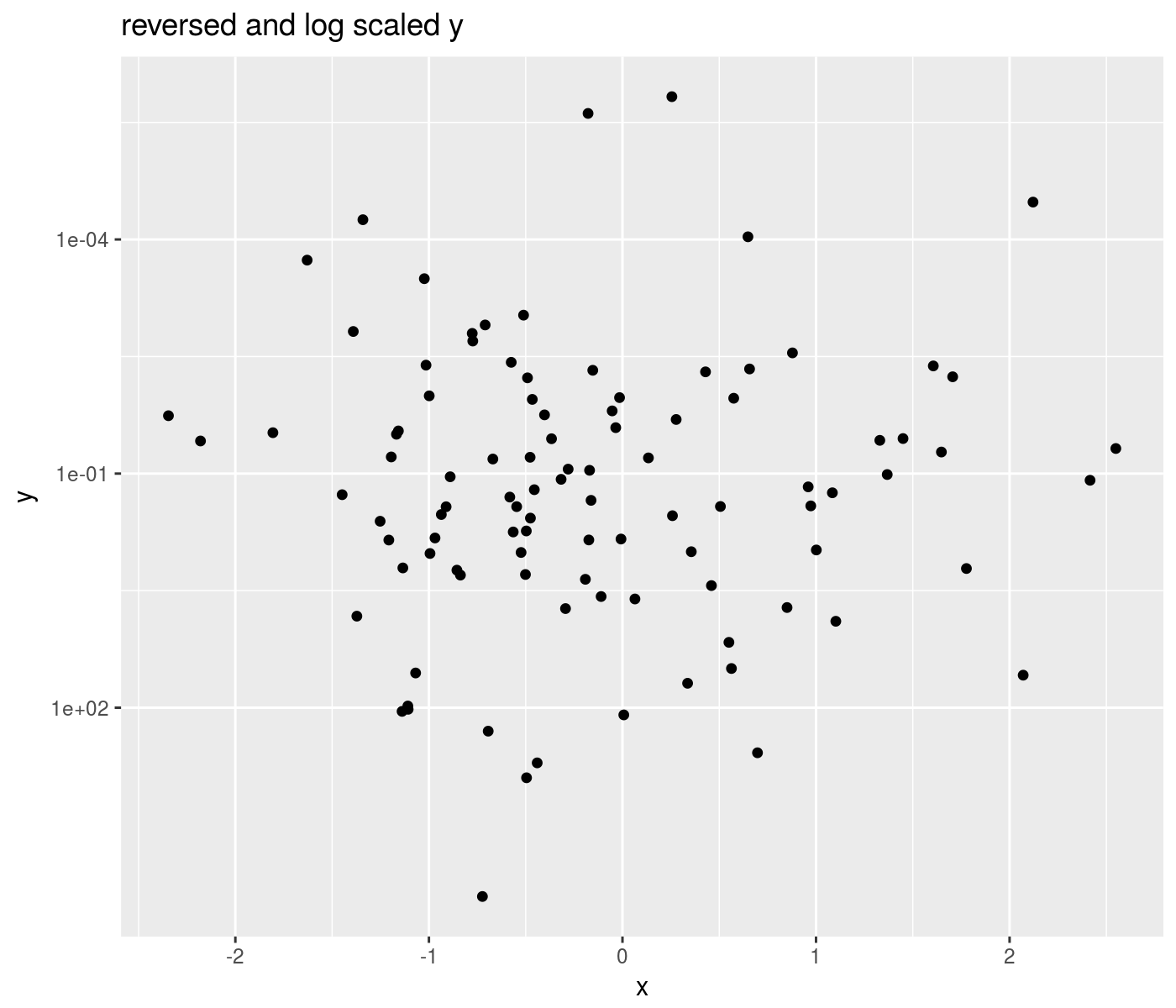
The %of% binary operator supports composition of scale transformations. This is most useful for composing reverse scales with other transforms:

library(ggplot2)
library(ggallin)

#  reverse and log scale
set.seed(1234)
ph <- ggplot(data.frame(x=rnorm(100),y=exp(rnorm(100,mean=-2,sd=4))),aes(x=x,y=y)) + 
  geom_point() + 
  scale_y_continuous(trans=scales::reverse_trans() %of% scales::log10_trans()) +
  labs(title='reversed and log scaled y')
print(ph)