Detecting Spatial Clustering Based on Connection Cost Between Grids.

habCluster

Based on landscape connectivity, use Community Detection Algorithm to find structure of raster and return a polygon representing the boundary of the clusters.

Installation

You can install the development version of habCluster from GitHub with:

# install.packages("devtools")
devtools::install_github("qiangxyz/habCluster")

Example

This is a basic example which shows you how to find the cluster of lands:

library(sf)
library(raster)
library(habCluster)

Read in habitat suitability index (HSI) data of wolf in Europe. The HSI values of the cells in the raster indicate how smoothly the wolfs can moved in the cells, and can be used to represent the connection between cells as habitat. The original value of HSI was 0 - 1.0 (float), yet was transformed to integers from 0 - 100 for reducing the file size.

hsi.file = system.file("extdata","wolf3_int.tif",package="habCluster")
wolf = raster(hsi.file)
# rescale raster value to 0 - 1
wolf = wolf / 100

Find habitat cluster using Leiden Algorithm. Raster for habitat suitability will be resampled to 40 km (40000 m), to reduce calculation amount. Set resolution_parameter to 0.0002 to control the cluster size. Note that the parameter of cellsize controls the spatial scale analysis is performed, while the parameter of resolution_parameter is used to control cluster size.

clst = cluster(wolf, method = cluster_leiden, cellsize = 40000, resolution_parameter = 0.0002, silent = FALSE)
#> 
#> resampling...
#> extracting edges...
#> create graph...
#> finding clusters...
#> preparing results...

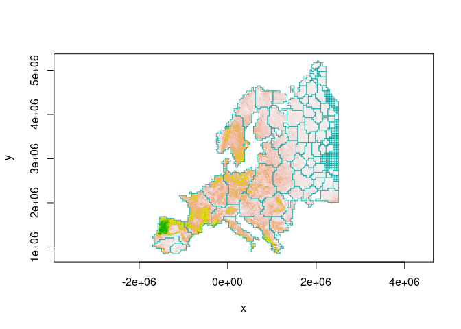
We can also embed plots, for example:

image(wolf, col = terrain.colors(100,rev = T), asp = 1)
boundary = clst$boundary
plot( boundary$geometry, add=TRUE, asp=1, border = "lightseagreen")

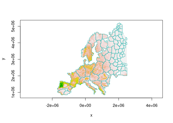
Or, we can discard small patches before plotting:

image(wolf, col = terrain.colors(100,rev = T), asp = 1)
boundary$area = as.numeric(st_area(boundary))
boundary = boundary[boundary$area > 40000*40000,]
plot(boundary$geometry, add=TRUE, asp=1, border = "lightseagreen")

Using stars to manipulate the raster will make the computation more quick:

hsi.file = system.file("extdata","wolf3_int.tif",package="habCluster")
wolf = read_stars(hsi.file)
wolf = wolf / 100
clst = cluster(wolf, method = cluster_leiden, cellsize = 40000, resolution_parameter = 0.0002, silent = FALSE)
#> 
#> resampling...
#> extracting edges...
#> create graph...
#> finding clusters...
#> preparing results...

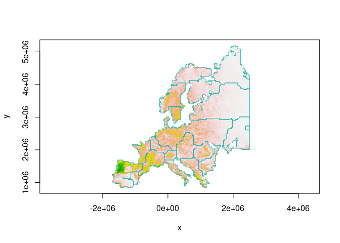
Leiden algorithm is not greedy, therefore the clusters are somehow random. We can use the Fast Greedy algorithm to avoid random results:

wolf = raster(hsi.file) / 100
clst = cluster(wolf, method = cluster_fast_greedy, cellsize = 40000)

image(wolf, col = terrain.colors(100,rev = T), asp = 1)
boundary = clst$boundary
plot( boundary$geometry, add=TRUE, asp=1, border = "lightseagreen")

How to Cite

Zhang,C., J. Li, B. Yang, Q. Dai*. (2022). habCluster: Identifying Geographical Boundary among Intraspecific Units Using Community Detection Algorithm in R. bioRxiv 2022.05.06.490926.