Set Data Visualization Using Hierarchies.
hierarchicalSets
What is this?
This is a package that facilitates hierarchical set analysis on large collections of sets.
OK, so what is Hierarchical Set Analysis?
Hierarchical Set Analysis is a way to investigate large numbers of sets. It consists of two things: A novel hierarchical clustering algorithm for sets and a range of visualizations that builds on top of the resulting clustering.
The clustering, in contrast to more traditional approaches to hierarchical clustering, does not rely on a derived distance measure between the sets, but instead works directly with the set data itself using set algebra. This has two results: First, it is much easier to reason about the result in a set context, and second, you are not forced to provide a distance if none exists (sets are completely independent). The clustering is based on a generalization of Jaccard similarity, called Set Family Homogeneity, that, in its simplest form, is defined as the size of the intersection of the sets in the family divided by the size of the union of the sets in the family. The clustering progresses by iteratively merging the set families that shows the highest set family homogeneity and is terminated once all remaining set family pairs have a homogeneity of 0. Note that this means that the clustering does not necessarily end with the all sets in one overall cluster, but possibly split into several hierarchies - this is intentional.
The visualizations uses the derived clustering as a scaffold to show e.g. intersection and union sizes of set combinations. By narrowing the number of set families to visualize to the branch points of the hierarchy the number of data points to show is linearly related to the number of sets under investigation, instead of the exponential if we chose to show everything. This means that hierachical set visualizations are much more scalable than e.g. UpSet and Radial Sets, at the cost of only showing combinations of the progressively most similar sets. Apart from intersection and union sizes there is a secondary analysis build into hierarchical sets that detects the elements not conforming to the imposed hierarchy. These outlying elements defines a subset of the universe that deviates from the rest and can be quite interesting - visualizations to investigate these are of course also provided.
Hierachical set analysis is obviuously sensible for collections of sets where a hierarchical structure makes sense, but even for set collection that does not obviously support a hierarchy, it can be interesting to look at how the different sets do, or do not, relate to each other.
How do I get it?
The stable version is available on CRAN with install.packages('hierarchicalSets'). Alternatively the development version can be obtained from GitHub using devtools:
# install.packages('devtools')
devtools::install_github('thomasp85/hierarchicalSets')
How do I use it?
hierarchicalSets comes with a toy dataset containing the followers of 100 prolific anonymous twitter users. To create the hierarchical clustering you use the create_hierarchy() function.
library(hierarchicalSets)
data('twitter')

twitSet <- create_hierarchy(twitter)
twitSet
#> A HierarchicalSet object
#>
#>                  Universe size: 28459
#>                 Number of sets: 100
#> Number of independent clusters: 6
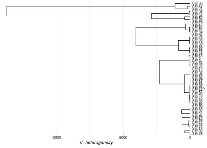
To simply have a look at the hierarchy you plot it:
plot(twitSet)

Here the x axis is encoded with the Set Family Heterogeneity which is the inverse of the homogeneity. It can thus be interpreted as the ratio of union to intersection size.
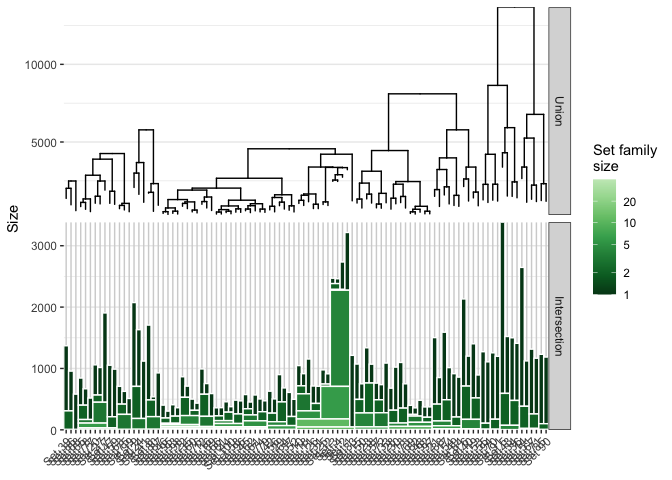
Usually we are interested in the direct numbers which can be provided with another plottype - the intersection stact
plot(twitSet, type = 'intersectStack', showHierarchy = TRUE)

We see that especially four sets are very similar, incidentally four of the largest sets. The rightmost cluster is interesting as well as we see it is held together by a very small overlap and that each individual set contains a lot of unique followers.
While it is expected that followers share some of the same patterns in terms of who they follow, it cannot be expected that they fully adhere to a single hierarchy. We can look at how sets are connected across the hierarchy by counting the number of elements they have in common that is not part of their closest shared set family. This can be shown using hierarchical edge bundles:
plot(twitSet, type = 'outlyingElements', quantiles = 0.8, alpha = 0.2)

It seems our four sets again draws attention to themselves by having strong connections to a range of other sets distant in terms of the clustering. Also it is obvious that there is two seperate groups of sets in terms of their deviation profile. There might be a secondary structure hidden within the outlying elements. Lets create a hierarchical set clustering based only on the outlying elements:
twitSet2 <- outlier_hierarchy(twitSet)
twitSet2
#> A HierarchicalSet object
#>
#>                  Universe size: 14657
#>                 Number of sets: 100
#> Number of independent clusters: 7
In this way it is possible to gradually shave off hierarchical structures, revealing the uncaptured relations of the prior analysis… Happy investigation!
Future work
Hierarchical Sets is static on purpose. I firmly belive that effective static plots are the foundation for any good visualization. You can always augment a static visualization with interactivity, but not all interactive visualizations can be used in a static way. That being said, it could be fun to experiment with said augmentation within a shiny app. Also, the implementation begins to struggle (just slow down actually) when being used with thousands of sets and millions of elements - some C++ wizardry might be warranted for such huge datasets.
Another nice idea I have in mind is to be able to keep set and element metadata within the HierarchicalSet object and seemlessly use it for plotting.